Work-in-progress 🚧
You are reading the work-in-progress first edition of Causal Inference in R. This chapter is mostly complete, but we might make small tweaks or copyedits.
You are reading the work-in-progress first edition of Causal Inference in R. This chapter is mostly complete, but we might make small tweaks or copyedits.
The propensity score workflow divides our work into two parts: the exposure model, or design phase, and the outcome model. The outcome model estimates the causal effect, building on the preparation in the design phase. For many outcome models, this stage is considerably simpler than the design phase: we fit a regression model as we normally would, but without the confounders. Instead of including confounders in the model, we either use a matched data set or weight the outcome model using propensity score weights. There’s a hiccup, though: the standard errors that come default with most regression toolkits do not account for the design phase. Thus, they will often produce incorrect uncertainty estimates. In this chapter, we transition to using matched and weighted data sets in outcome models and explore several methods for calculating standard errors.
When fitting an outcome model on matched data sets, we subset the original data to only those who were matched and then fit a model on these data as we would otherwise. That’s it! For example, re-performing the matching as we did in Section 8.2, we extract the matched observations in a data set called matched_data.
library(broom)
library(touringplans)
library(MatchIt)

seven_dwarfs_9 <- seven_dwarfs_train_2018 |>
  filter(wait_hour == 9)

matchit_obj <- matchit(
  park_extra_magic_morning ~ park_ticket_season +
    park_close +
    park_temperature_high,
  data = seven_dwarfs_9
)
matched_data <- get_matches(matchit_obj)
Remember that, with matching, we are trying to find a subset of the data where the assumptions of causal inference, particularly exchangeability, hold. If we have succeeded in doing so, we can compare the differences in wait times between the groups without additional covariates, much as we can in a randomized trial. There are other good reasons to include covariates in the outcome model, including improved precision, heterogeneous treatment effects, and, as we will see, to get the correct standard errors, but for now, we will focus on the simple question at hand: Does having Extra Magic Mornings change the posted wait time between 9 AM and 10 AM?
To answer this question, let’s fit a linear regression with the matched data set. Here, we have the posted wait times as the outcome and Extra Magic Mornings as the exposure.
matched_outcome <- lm(
  wait_minutes_posted_avg ~ park_extra_magic_morning,
  data = matched_data
)

matched_outcome |>
  tidy(conf.int = TRUE)
# A tibble: 2 × 7
term estimate std.error statistic p.value conf.low
<chr> <dbl> <dbl> <dbl> <dbl> <dbl>
1 (Inte… 67.0 2.37 28.3 1.94e-54 62.3
2 park_… 7.87 3.35 2.35 2.04e- 2 1.24
# ℹ 1 more variable: conf.high <dbl>Recall that, by default, MatchIt finds pairs of observations that help us estimate an average treatment effect among the treated. This means among days that have Extra Magic Mornings, the expected impact of having Extra Magic Mornings on the average posted wait time between 9 AM and 10 AM is 7.9 minutes (95% CI: 1.2-14.5).
Fitting a regression with matched data is straightforward; however, the lm() function doesn’t know that we pre-processed the data with MatchIt. In doing so, we induced a dependence between pairs of matches. We’ll have to account for that clustering to get correct standard errors (Abadie and Spiess 2022). What we need to do is a little more complex than for weighting—and, in fact, will build on the approaches we use for IPW—so we’ll pause on that fix until Section 11.4.
Using propensity score weights in outcome models requires only one additional step: instructing the regression function to use the weights when fitting the model.
In our previous examples, we used ATE weights; however, here we will use ATT weights so the effect estimate is comparable to the matching-based analysis above. Our workflow is identical to the previous way we calculated the propensity score weights, except we use propensity::wt_att().
library(propensity)

propensity_model <- glm(
  park_extra_magic_morning ~ park_ticket_season +
    park_close +
    park_temperature_high,
  data = seven_dwarfs_9,
  family = binomial()
)

seven_dwarfs_9_with_wt <- propensity_model |>
  augment(type.predict = "response", data = seven_dwarfs_9) |>
  mutate(w_att = wt_att(.fitted, park_extra_magic_morning))
We can fit a weighted outcome model by using the weights argument. Note that, with weighting, we still use the entire data set for the data argument (seven_dwarfs_9_with_wt), unlike in matching, where we only use the matched subset. We instead smoothly combine information from each observation to create a pseudo-population in which (we hope) there is no confounding.
weighted_outcome <- lm(
  wait_minutes_posted_avg ~ park_extra_magic_morning,
  data = seven_dwarfs_9_with_wt,
  weights = w_att
)

weighted_outcome |>
  tidy()
# A tibble: 2 × 5
term estimate std.error statistic p.value
<chr> <dbl> <dbl> <dbl> <dbl>
1 (Intercept) 68.7 1.45 47.3 1.69e-154
2 park_extra_ma… 6.23 2.05 3.03 2.62e- 3weights
MatchIt returns a data frame that includes a weights variable. In the example above, all the weights are 1:
unique(matched_data$weights)[1] 1However, some matching schemes, such as full matching, also use weights. Since the weights will either be useful (as in full matching) or benign (as in equal weights for everyone), the authors of the MatchIt package recommend always setting weights = weights in the outcome model. In our earlier case, we could also fit:
matched_outcome <- lm(
  wait_minutes_posted_avg ~ park_extra_magic_morning,
  data = matched_data,
  weights = weights
)
Again, these weights are all 1, so we get identical results. However, if you are considering other matching approaches, it’s a good defensive practice to ensure you specify the outcome model correctly. Matching itself can be thought of as an extreme form of weighting where everyone with a match gets a non-zero weight and everyone without a match gets a weight of 0, so it’s also logically consistent.
Using weighting, we estimate that among days that have Extra Magic Mornings, the expected impact of having Extra Magic Mornings on the average posted wait time between 9 AM and 10 AM is 6.2 minutes.
group_by() and summarize(), revisted
In this simple example, the weighted outcome model is equivalent to the difference between the weighted means. The weighted population is a pseudo-population where there is no confounding by the variables in the propensity score. Philosophically and practically, we can perform calculations directly from the data in this population.
In this case, weighted.mean() will help us calculate the means among the pseudo-population.
wt_means <- seven_dwarfs_9_with_wt |>
  group_by(park_extra_magic_morning) |>
  summarize(
    average_wait = weighted.mean(wait_minutes_posted_avg, w = as.numeric(w_att))
  )

wt_means
# A tibble: 2 × 2
park_extra_magic_morning average_wait
<dbl> <dbl>
1 0 68.7
2 1 74.9The difference is 6.23, the same as the weighted outcome model. Causal inference with group_by() and summarize() works just fine now, since we’ve already accounted for confounding in the weights.
While this approach will give us the desired point estimate, the default output from the lm() function for the uncertainty (standard errors and confidence intervals) is incorrect. The reason for this problem is slightly different than matching: lm() thinks that the values we pass to the weights argument are fixed weights, as in frequency weights. However, our weights are not fixed; they are estimated. The estimate of the weights themselves introduces uncertainty that we need to bring downstream to the uncertainty around the point estimate.
Inverse probability weighting is a two-step estimator: first, we fit a regression for the exposure and generate weights from the propensity score, then we use those weights to fit a regression for the outcome. To correctly specify the uncertainty in the second model, we need to include the uncertainty from the first one. Much of this chapter is focused on statistical inference. While causal inference is the set of tools that we’ve used so far to make causal effect estimation possible, statistical inference is the more general toolkit of standard errors, confidence intervals, and hypothesis tests, built on sampling distributions of estimators. It’s the kind of inference normally taught in a statistics class. Like the distinction between description, prediction, and causal inference, these are separate but complementary ideas: we use statistical inference to test if our causal estimates have a meaningful statistical interpretation, and as we have seen, interpreting statistical results such as estimation or hypothesis testing from a causal perspective requires causal assumptions.
There are three ways to estimate the uncertainty for IPW:
The first option can be computationally intensive, but it should get you the correct estimates. The bootstrap is also a general solution to many problems of causal inference uncertainty, so knowing it is very useful. The second option is computationally easier but tends to overestimate or underestimate the variability. The third option is both correct and fast to compute; however, it is mathematically more complicated, usually relying on the calculus of M-Estimation to calculate (Stefanski and Boos 2002). We’ll use the tools in propensity’s ipw() function to compute the correct sandwich estimator. It’s also implemented in WeightIt, PSweight, and a few other tools.
We used the bootstrap in Chapter 2 to estimate the uncertainty around the causal effect estimate of mosquito nets on malaria risk (see also Appendix A for a detailed exploration of the bootstrap). The algorithm is identical here.
First, we’ll create a function to run the analysis once on a sample of the data.
fit_ipw <- function(.split, ...) {
  # get bootstrapped data frame
  .df <- as.data.frame(.split)

  # fit propensity score model
  propensity_model <- glm(
    park_extra_magic_morning ~ park_ticket_season +
      park_close +
      park_temperature_high,
    data = seven_dwarfs_9,
    family = binomial()
  )

  # calculate inverse probability weights
  .df <- propensity_model |>
    augment(type.predict = "response", data = .df) |>
    mutate(
      wts = wt_att(
        .fitted,
        park_extra_magic_morning,
        exposure_type = "binary"
      )
    )

  # fit correctly bootstrapped ipw model
  lm(
    wait_minutes_posted_avg ~ park_extra_magic_morning,
    data = .df,
    weights = wts
  ) |>
    tidy()
}
Then use rsample to bootstrap the data set and apply the function to each bootstrap sample.
library(rsample)

# fit ipw model to bootstrapped samples
bootstrapped_seven_dwarfs <- bootstraps(
  seven_dwarfs_9,
  times = 1000,
  apparent = TRUE
)

ipw_results <- bootstrapped_seven_dwarfs |>
  mutate(boot_fits = map(splits, fit_ipw))

ipw_results
# Bootstrap sampling with apparent sample
# A tibble: 1,001 × 3
splits id boot_fits
<list> <chr> <list>
1 <split [354/131]> Bootstrap0001 <tibble [2 × 5]>
2 <split [354/124]> Bootstrap0002 <tibble [2 × 5]>
3 <split [354/133]> Bootstrap0003 <tibble [2 × 5]>
4 <split [354/126]> Bootstrap0004 <tibble [2 × 5]>
5 <split [354/143]> Bootstrap0005 <tibble [2 × 5]>
6 <split [354/135]> Bootstrap0006 <tibble [2 × 5]>
7 <split [354/124]> Bootstrap0007 <tibble [2 × 5]>
8 <split [354/131]> Bootstrap0008 <tibble [2 × 5]>
9 <split [354/133]> Bootstrap0009 <tibble [2 × 5]>
10 <split [354/134]> Bootstrap0010 <tibble [2 × 5]>
# ℹ 991 more rowsAfter applying fit_ipw() to each replicate of the data set, we obtain a distribution of effect estimates.
ipw_results |>
  mutate(
    estimate = map_dbl(
      boot_fits,
      \(.fit) {
        .fit |>
          filter(term == "park_extra_magic_morning") |>
          pull(estimate)
      }
    )
  ) |>
  ggplot(aes(estimate)) +
  geom_histogram(bins = 30, fill = "#D55E00FF", color = "white", alpha = 0.8) +
  theme_minimal()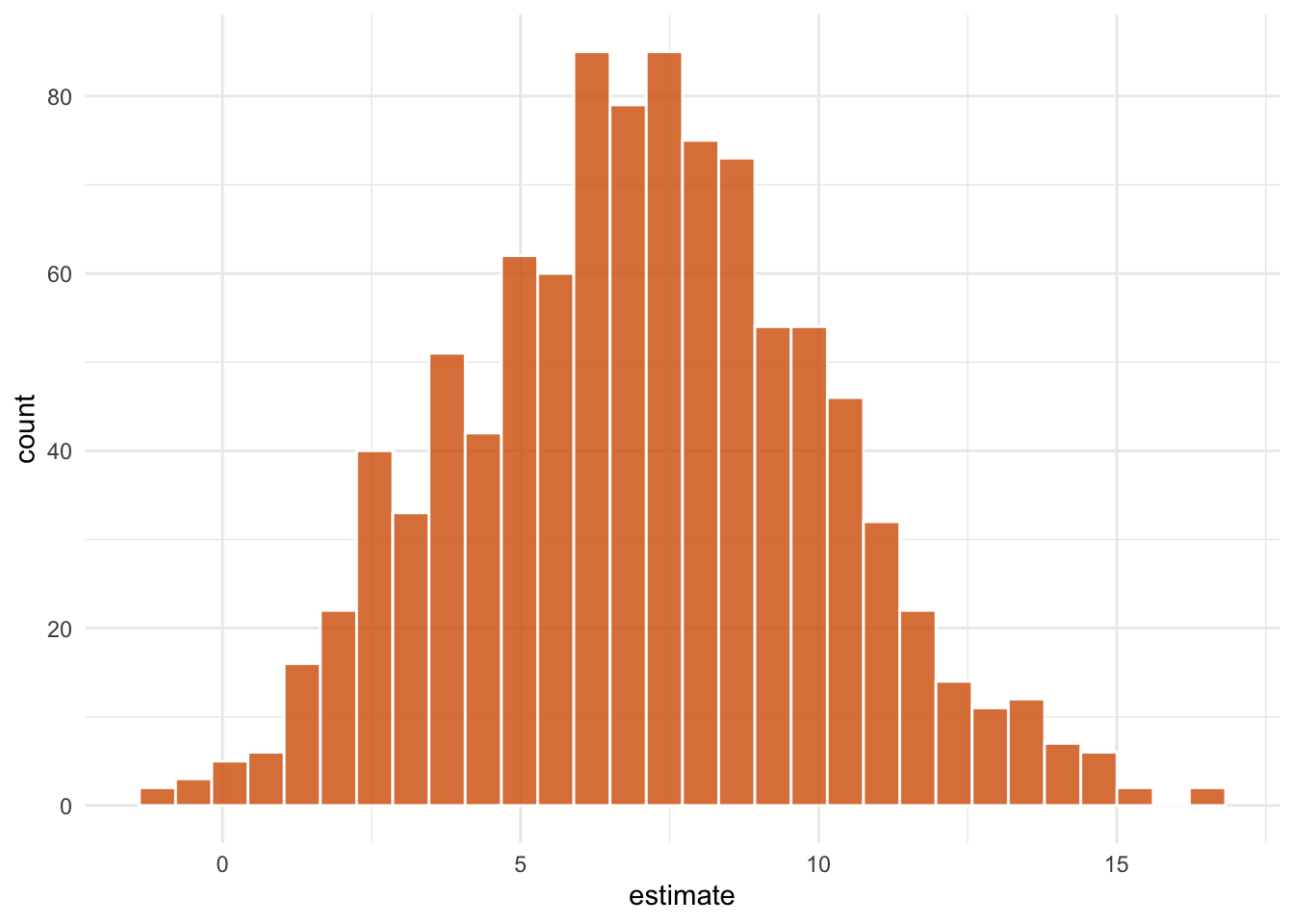
park_extra_magic_morning coefficient. The spread captures the combined uncertainty from both estimation steps and is the basis for the bootstrap confidence interval reported below.
Finally, calculate the confidence intervals from this distribution using one of rsample’s int_*() functions (here, we use int_t() to calculate a simple t-statistic-based CI).
# get t-based CIs
boot_estimate <- int_t(ipw_results, boot_fits) |>
  filter(term == "park_extra_magic_morning")
boot_estimate
# A tibble: 1 × 6
term .lower .estimate .upper .alpha .method
<chr> <dbl> <dbl> <dbl> <dbl> <chr>
1 park_extra_ma… 0.0116 6.75 11.4 0.05 studen…Now that we have incorporated the uncertainty we introduced estimating the propensity scores, we can say more correctly: we estimate that among days that have Extra Magic Mornings, the expected impact of having Extra Magic Mornings on the average posted wait time between 9 AM and 10 AM is 6.8 minutes, 95% CI (0, 11.4).
The bootstrap works well for a wide variety of problems. However, it’s both verbose and computationally intensive. Let’s now take a look at two approaches using robust sandwich estimators.
The sandwich estimator gets its name from the form of the variance it calculates: a “meat” matrix built from the variability of each observation’s residuals, sandwiched between two copies of a “bread” matrix that comes from the design of the model (the predictors and weights). When the model’s assumptions hold, the bread and meat combine to give the usual model-based variance; when they don’t—as with IPW weights—the sandwich form still gives a consistent variance estimate. That’s why these are called “robust” standard errors.
Many packages implement sandwich estimators for variance, but let’s first compute it by hand with the sandwich package and compare it to the variance lm() gives us by default. vcov() returns the variance-covariance matrix that tidy() and summary() use under the hood to compute their standard errors. It treats the weights we passed as fixed, which, in our case, they aren’t.
vcov(weighted_outcome) (Intercept)
(Intercept) 2.111
park_extra_magic_morning -2.111
park_extra_magic_morning
(Intercept) -2.111
park_extra_magic_morning 4.223sandwich() returns a matrix of the same shape, where the diagonal entries are the variances of each coefficient.
                         (Intercept)
(Intercept)                    1.488
park_extra_magic_morning      -1.488
                         park_extra_magic_morning
(Intercept)                                -1.488
park_extra_magic_morning                    8.727
The two matrices disagree. For the treatment coefficient, the sandwich variance (8.727) is more than double the model-based one (4.223), so the model-based SE understates the uncertainty around the treatment effect. For the intercept, the sandwich version is smaller. We can then use this to construct a robust confidence interval.
robust_ci <- tibble(
  estimate = coef(weighted_outcome)[2],
  # calculate the robust standard error
  # from the robust variance
  robust_se = sqrt(sandwich(weighted_outcome)[2, 2]),
  # and use the SE to calculate the 95% CI
  conf.low = estimate - 1.96 * robust_se,
  conf.high = estimate + 1.96 * robust_se
)

robust_ci
# A tibble: 1 × 4
estimate robust_se conf.low conf.high
<dbl> <dbl> <dbl> <dbl>
1 6.23 2.95 0.438 12.0Now, let’s try to say our interpretation again, this time using the sandwich estimator as the basis for the uncertainty: we estimate that among days that have Extra Magic Mornings, the expected impact of having Extra Magic Mornings on the average posted wait time between 9 AM and 10 AM is 6.2 minutes, 95% CI (0.4, 12).
The variance returned by a bare call to sandwich() is sometimes called HC0. The “HC” part stands for “heteroskedasticity-consistent” because these techniques were originally developed to address heteroskedasticity in regression fits. HC0 tends to be downwardly biased in small samples because least-squares residuals systematically understate the true errors, especially at high-leverage points. A family of refinements has accumulated over the years (Mansournia et al. 2021). HC1 applies a degrees-of-freedom correction of \(n / (n - k)\). HC2 and HC3 instead inflate each squared residual to undo the shrinkage caused by leverage—HC2 by \(1 / (1 - h_{ii})\) and HC3 by \(1 / (1 - h_{ii})^2\), where \(h_{ii}\) is the leverage of observation \(i\). HC3 approximates the jackknife, another form of resampling used to calculate variance. HC4 and successors push the leverage adjustment further at extreme points.
The sandwich() function can compute any of these variants if you swap in the HC meat estimator: sandwich(model, meat. = meatHC, type = "HC3"). The convenience wrapper sandwich::vcovHC(model) does the same thing and defaults to HC3, which many authors recommend as a reasonable starting point for most analyses (Long and Ervin 2000).
Alternatively, we can use marginaleffects to compute the same quantity from the fitted model, along with robust standard errors built in.
library(marginaleffects)

avg_comparisons(
  weighted_outcome,
  variables = "park_extra_magic_morning",
  vcov = "HC3"
)
 Estimate Std. Error    z Pr(>|z|)   S 2.5 % 97.5 %
     6.23          3 2.08   0.0378 4.7  0.35   12.1

Term: park_extra_magic_morning
Type: response
Comparison: 1 - 0
avg_comparisons() returns a marginal effect: the average of \(\hat{Y}(1) - \hat{Y}(0)\) across the observed covariate distribution. We’ll come back to this subject, and marginaleffects, in more detail in Chapter 13. Passing vcov = "HC3" requests the HC3 variance estimator from the previous callout.
Another way to fit the same weighted outcome model is via the survey package, which treats the IPW weights as survey sampling weights and adjusts the standard errors accordingly. Historically, many propensity score analyses in R used this approach, so you might see it out in the wild. You wrap the data and weights in a design object and then fit the model with svyglm():
library(survey)

des <- svydesign(
  ids = ~1,
  weights = ~w_att,
  data = seven_dwarfs_9_with_wt
)

svyglm(wait_minutes_posted_avg ~ park_extra_magic_morning, des) |>
  tidy(conf.int = TRUE)
# A tibble: 2 × 7
term estimate std.error statistic p.value conf.low
<chr> <dbl> <dbl> <dbl> <dbl> <dbl>
1 (Int… 68.7 1.22 56.2 6.14e-178 66.3
2 park… 6.23 2.96 2.11 3.60e- 2 0.410
# ℹ 1 more variable: conf.high <dbl>The standard errors reported by svyglm() are based on the same family of robust sandwich estimators, so the results are comparable to the manual approach above.
The correct sandwich estimator also accounts for the uncertainty in the propensity score model. propensity’s ipw() function uses this approach. ipw() is a bring-your-own-model (BYOM) inverse probability weighted estimator. Rather than fitting the two regressions for you, you fit them yourself, then supply them to ipw(). This allows you to retain control—and, crucially, diagnostic ownership—over the regression fits.
We already fit both models, so let’s pass them to ipw().
results <- ipw(propensity_model, weighted_outcome)
results
Inverse Probability Weight Estimator
Estimand: ATT
Propensity Score Model:
Call: glm(formula = park_extra_magic_morning ~ park_ticket_season +
park_close + park_temperature_high, family = binomial(),
data = seven_dwarfs_9)
Outcome Model:
Call: lm(formula = wait_minutes_posted_avg ~ park_extra_magic_morning,
data = seven_dwarfs_9_with_wt, weights = w_att)
Estimates:
estimate std.err z ci.lower ci.upper
diff 6.23 2.34 2.66 1.64 10.8
conf.level p.value
diff 0.95 0.0078 **
---
Signif. codes:
0 '***' 0.001 '**' 0.01 '*' 0.05 '.' 0.1 ' ' 1We can also collect the results in a data frame.
results |>
  as.data.frame()
effect estimate std.err z ci.lower ci.upper
1 diff 6.228 2.339 2.663 1.644 10.81
conf.level p.value
1 0.95 0.007753IPW is a two-step estimator: fit a propensity model, then run a weighted outcome regression. The naive sandwich estimator above treats the propensity scores as known constants and ignores the propensity-estimation step entirely. Two routes recover a closed-form variance that accounts for both steps.
M-estimation (Stefanski and Boos 2002; Ross et al. 2024; Williamson, Forbes, and White 2014) stacks the two stages into a single system of estimating equations: the score equations from the propensity model and those from the weighted outcome regression, solved simultaneously for the combined parameter vector. The joint estimator’s variance is the usual sandwich built from that whole system, so propensity-stage uncertainty propagates into the outcome-stage variance automatically.
Linearization (Kostouraki et al. 2024) works one observation at a time. Each observation’s contribution to the variance is written as a Taylor expansion in the propensity-score coefficients and decomposed into two pieces. The first is the influence-function contribution from the weighted regression alone, equal to what the naive sandwich computes. The second is a correction term that propagates that observation’s role in fitting the propensity model into the outcome estimate via the chain rule. Adding the two pieces and averaging gives a closed-form variance.
The two approaches are connected. Under a logit propensity model, linearization and M-estimation formulas are algebraically identical (Kostouraki et al. 2024).
Now that we’ve seen some approaches for correcting IPW estimators, let’s return to matching. The simple model wait_minutes_posted_avg ~ park_extra_magic_morning omits the matching covariates. Matching pairs units with similar values of the covariates, so the paired residuals are correlated. lm() and a bare call to sandwich() both treat observations as independent and miss this correlation. Naive standard errors are valid only when matching is done without replacement, and the outcome model is correctly specified (Abadie and Spiess 2022). Outside that case, the SEs are biased.
There are three fixes.
The most direct approach is to include the matching covariates in the outcome model with the right functional form. Correctly specifying the model removes the omitted-variable signal from the residuals, and naive SEs become valid. The catch is that we now need to avoid misspecifying the functional form of all covariates used for matching in the outcome model. We can never be certain that we have achieved this. The other two fixes correct the SE without including more variables in the outcome model, and so they are a more forgiving approach.
The second solution is a cluster-robust standard error clustered within matched pairs. get_matches() returns a subclass column identifying each pair, which we pass to sandwich::vcovCL() as the cluster argument (as a formula) to compute the cluster-robust variance.
vcl <- vcovCL(matched_outcome, cluster = ~subclass)

robust_ci <- tibble(
  estimate = coef(matched_outcome)[["park_extra_magic_morning"]],
  robust_se = sqrt(vcl["park_extra_magic_morning", "park_extra_magic_morning"]),
  conf.low = estimate - 1.96 * robust_se,
  conf.high = estimate + 1.96 * robust_se
)

robust_ci
# A tibble: 1 × 4
estimate robust_se conf.low conf.high
<dbl> <dbl> <dbl> <dbl>
1 7.87 2.73 2.52 13.2marginaleffects::avg_comparisons() computes the same cluster-robust SE by passing ~subclass to vcov.
avg_comparisons(
  matched_outcome,
  variables = "park_extra_magic_morning",
  vcov = ~subclass,
  newdata = filter(matched_data, park_extra_magic_morning == 1)
)
 Estimate Std. Error    z Pr(>|z|)   S 2.5 % 97.5 %
     7.87       2.73 2.88  0.00393 8.0  2.52   13.2

Term: park_extra_magic_morning
Type: response
Comparison: 1 - 0
Since we are targeting the ATT, we also need to filter the data down to the treated before calculating the average comparisons; we’ll come back to that topic in Chapter 13.
The third solution is a cluster bootstrap: resample whole matched pairs as units rather than rows, leaving the matching itself fixed. In contrast to the bootstrap for IPW, we do not re-run matchit() within the bootstrap. The standard bootstrap is theoretically invalid for nearest-neighbor matching estimators (Abadie and Imbens 2008); instead, we should resample matched pairs (Abadie and Spiess 2022). rsample::group_bootstraps() creates this pair-level bootstrap when we pass it subclass as the group variable; the function-then-bootstrap pattern mirrors Section 11.3.1, except that we do not refit the MatchIt object.
fit_matched <- function(.split, ...) {
  .df <- as.data.frame(.split)
  lm(
    wait_minutes_posted_avg ~ park_extra_magic_morning,
    data = .df
  ) |>
    tidy()
}

cluster_boots <- group_bootstraps(
  matched_data,
  group = subclass,
  times = 1000,
  apparent = TRUE
)

cluster_results <- cluster_boots |>
  mutate(boot_fits = map(splits, fit_matched))

int_t(cluster_results, boot_fits) |>
  filter(term == "park_extra_magic_morning")
# A tibble: 1 × 6
term .lower .estimate .upper .alpha .method
<chr> <dbl> <dbl> <dbl> <dbl> <chr>
1 park_extra_ma… 2.50 7.90 13.3 0.05 studen…In the example we’ve taken up, the outcome, posted wait times, is continuous. Using weighted linear regression, the ATE and friends are estimated as differences in means. A difference in means is a valuable effect to estimate, but it’s not the only one. Let’s say we use ATT weights and weight an outcome regression to calculate the relative change in posted wait time. The relative change is still a treatment effect among the treated, but it’s on a relative scale. The important part is that the weights allow us to average over the covariates of the treated for whichever specific estimand we’re trying to estimate. Sometimes, when people say something like “the average treatment effect,” they’re referring to the difference in mean outcomes across the whole sample, so it’s good to be specific.
What about other types of outcomes that are not continuous? For example, let’s discretize the continuous posted wait time into a binary indicator of whether the average wait exceeded 60 minutes. Discretizing a continuous variable is generally a bad idea—we’re sacrificing information by dichotomizing the outcome—but we’ll use it as an example to show how to approach a problem that has a binary outcome.
seven_dwarfs_9_with_wt <- seven_dwarfs_9_with_wt |>
  mutate(wait_over_60 = wait_minutes_posted_avg > 60)
For binary outcomes, there are three standard options: the risk ratio, the risk difference, and the odds ratio. For a binary outcome, we calculate the average probability for each treatment group. Let’s call these \(p_{\text{untreated}}\) and \(p_{\text{treated}}\). When we’re working with these probabilities, calculating the risk difference and risk ratio is simple:
By “risk”, we mean the risk of an outcome. That assumes the outcome is negative, like developing a disease. Sometimes, you’ll hear these described as the “response ratio” or the “response difference.” A more general way to think about these is as the difference in, or the ratio of, the probabilities of the outcome.
The odds for a probability are calculated as \(p / (1 - p)\), so the odds ratio is:
When outcomes are rare, \((1 - p)\) approaches 1, and odds ratios approximate risk ratios. The rarer the outcome, the closer the approximation.
One feature of the logistic regression model is that the coefficients are log-odds ratios; exponentiating them yields odds ratios. However, when using logistic regression, you can also work with predicted probabilities to calculate risk differences and ratios, as we’ll see in Chapter 13.
Just as with continuous outcomes, we can target each of these estimands to a different subset of the population, e.g., the risk ratio among the untreated, the odds ratio among the evenly matchable, and so on.
These options also extend to categorical outcomes. There are different ways of organizing them depending on the nature of the categorical variables. An effect that’s commonly estimated for non-ordinal categorical variables is a series of odds ratios, with one level of the outcome serving as the reference level (e.g., ORs for 1 vs. 2, 1 vs. 3, and so on). Multinomial regression models, such as nnet::multinom(), can produce these log-odds ratios as coefficients, extending logistic regression. For ordinal outcomes, ordinal logistic regression, as implemented in MASS::polr(), estimates a series of log-odds ratios that compare each previous value of the outcome. Like logistic regression, you are not limited to odds ratios with these extensions, as you can work with the predicted probabilities of each category to calculate the effect you’re interested in.
Case-control studies are a typical design in epidemiology, in which participants are sampled by outcome status (Schlesselman 1982). Cases with the outcome are recruited, and controls are sampled from the population from which the cases come. These types of studies are used when outcomes are rare. They can also be faster and cheaper than studies that follow people from the time of exposure.
Because of how sampling happens in case-control studies, you don’t have a baseline risk because you don’t have all the individuals who did not have the outcome. Interestingly, you can still recover the odds ratio. When outcomes are rare, odds ratios approximate risk ratios. You cannot, however, calculate the risk difference.
Absolute measures, such as risk differences, and relative measures, such as the risk and odds ratios, offer different perspectives on the treatment effect. Depending on the baseline probability of the outcome, absolute and relative measures might lead you to different conclusions.
Consider a rare outcome with a baseline probability of 0.0001, a rate of 1 event per 10,000 observations. That’s the probability for the unexposed. Let’s say the exposed have a probability of 0.0008 of the outcome. That’s 8 times greater than the unexposed, a substantial relative effect. But it’s only 0.0007 on the absolute scale.
Now, consider a more common outcome with a baseline probability of 0.20. The exposed group has a probability of the outcome of 0.40. Now, the relative risk is 2, while the risk difference is 0.20. Although the relative effect is much smaller, it creates more outcome events because the outcome is more prevalent.
The effect of smoking on health is an excellent example of this. As we know, smoking drastically increases the relative risk of lung cancer. But lung cancer is a pretty rare disease. Smoking also increases the risk of heart disease, although the relative effect is not nearly as high as lung cancer. However, heart disease is much more prevalent. More people die of smoking-related heart disease than they do of lung cancer because of the absolute change in risk. Both the absolute and relative perspectives are valid and useful.
Another perspective on the difference in probabilities is the number needed to treat (NNT) measure. It’s simply the inverse of the risk difference and represents the number of exposed individuals needed to prevent or cause one outcome.
Consider a product with a baseline purchase probability of 5%, meaning that 5 in 100 people will buy it. A marketing team creates an ad, and those who see it have a 7% chance of buying the product. The absolute difference in the probability of buying the product is 0.02, so \(1 / 0.02 = 50\) people need to see the ad to increase the number of purchases by 1.
The NNT is an imperfect measure because of its simplicity, but it offers another perspective on what the treatment effect actually means in practice.
Odds ratios are convenient because of their connection to logistic regression. They also have a peculiar quality: they are non-collapsible. Non-collapsibility means that, when you compare odds ratios in the whole sample (marginal) versus among subgroups (conditional), the marginal odds ratio is not a weighted average of the conditional odds ratio (Didelez and Stensrud 2021; Greenland 2021a, 2021b). This is not a property that, for instance, the risk ratio has. Let’s look at an example.
Say we have an outcome, an exposure, and a covariate. exposure causes outcome, as does covariate1. But covariate does not cause exposure; it’s not a confounder. In other words, the effect estimate of exposure on outcome should be the same whether or not we account for covariate.
library(ggdag)
dagify(
  outcome ~ exposure + covariate,
  coords = time_ordered_coords()
) |>
  ggdag(use_text = FALSE) +
  geom_dag_text_repel(aes(label = name), box.padding = 1.8, direction = "x") +
  theme_dag()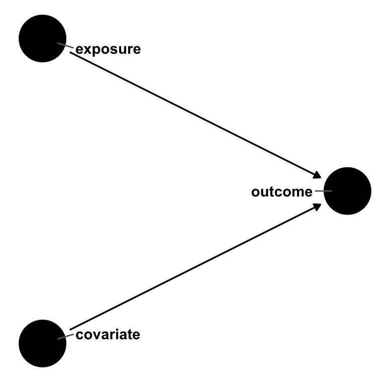
outcome, exposure, and covariate. exposure and covariate both cause outcome, but there is no relationship between exposure and covariate. In a logistic regression, the odds ratio for exposure will be non-collapsible over strata of covariate.
Let’s simulate this.
odds_ratio <- function(tbl) {
  or <- (tbl[2, 2] * tbl[1, 1]) / (tbl[1, 2] * tbl[2, 1])
  round(or, digits = 2)
}

risk_ratio <- function(tbl) {
  risk_exposed <- tbl[2, 2] / (tbl[2, 2] + tbl[2, 1])
  risk_unexposed <- tbl[1, 2] / (tbl[1, 2] + tbl[1, 1])
  round(risk_exposed / risk_unexposed, digits = 2)
}

marginal_table <- table(exposure, outcome)
marginal_or <- odds_ratio(marginal_table)
marginal_rr <- risk_ratio(marginal_table)
conditional_tables <- table(exposure, outcome, covariate)
conditional_or_0 <- odds_ratio(conditional_tables[,, 1])
conditional_or_1 <- odds_ratio(conditional_tables[,, 2])
conditional_rr_0 <- risk_ratio(conditional_tables[,, 1])
conditional_rr_1 <- risk_ratio(conditional_tables[,, 2])
First, let’s look at the relationship between exposure and outcome for everyone.
table(exposure, outcome) outcome
exposure 0 1
0 2036 3021
1 1115 3828We can calculate the odds ratio using this frequency table: ((3828 * 2036) / (3021 * 1115)) = 2.31.
This odds ratio is the same as the one we get with logistic regression when we exponentiate the coefficients.
# A tibble: 2 × 5
  term        estimate std.error statistic  p.value
  <chr>          <dbl>     <dbl>     <dbl>    <dbl>
1 (Intercept)     1.48    0.0287      13.8 4.33e-43
2 exposure        2.31    0.0445      18.9 2.87e-79
This is slightly off from the simulation model’s coefficient for exp(1). We get closer when we add in covariate.
# A tibble: 3 × 5
  term        estimate std.error statistic   p.value
  <chr>          <dbl>     <dbl>     <dbl>     <dbl>
1 (Intercept)    0.614    0.0378     -12.9 6.07e- 38
2 exposure       2.78     0.0493      20.7 1.33e- 95
3 covariate      7.39     0.0529      37.8 1.04e-312
covariate is not a confounder, so, by rights, it shouldn’t affect the exposure effect estimate. Let’s look at the conditional odds ratios by covariate.
table(exposure, outcome, covariate), , covariate = 0
outcome
exposure 0 1
0 1572 986
1 951 1589
, , covariate = 1
outcome
exposure 0 1
0 464 2035
1 164 2239The odds ratio for those with covariate = 0 is 2.66. For those with covariate = 1, it’s 3.11. The marginal odds ratio, 2.31, is smaller than both of these!
The marginal risk ratio is 1.3. The risk ratio for those with covariate = 0 is 1.62. For those with covariate = 1, it’s 1.14. In this case, the marginal risk ratio is a weighted average that can be collapsed across strata of the covariate (Huitfeldt, Stensrud, and Suzuki 2019).
It’s tempting to think you need to include a covariate because the odds ratio changes when you add it, and it’s closer to the model coefficient from the simulation. An important detail here is that non-collapsibility is not bias. Some authors describe it as omitted-variable bias, but the marginal and conditional odds ratios are both correct because covariate is not a confounder. They are, instead, different estimands. The conditional odds ratio is the OR conditional on covariate. To meaningfully compare it to other odds ratios, those odds ratios also need to condition on covariate. Non-collapsibility is a numerical property of odds; rather than creating bias, it creates a slightly more nuanced interpretation. The exact way non-collapsibility behaves also depends on whether the data-generating mechanism occurs on the additive or multiplicative scale; on the multiplicative scale (as in our simulation), removing a variable strongly related to the outcome changes the effect estimate, while on the additive scale, adding a variable strongly related to the outcome changes the effect, albeit on a smaller scale (Whitcomb and Naimi 2020). Instead of worrying about which version of the odds ratio is right, we recommend focusing on confounders, which are necessary for unbiased estimates, and predictors of the outcome, which are helpful for variance reduction.
Much ink has been spilled about the odds ratio versus the risk ratio and the relative versus absolute scale. We suggest that, for binary outcomes, you present all three measures (the odds ratio, the risk ratio, and the risk difference) together with the baseline probability of the outcome. Each offers a different perspective on the causal effect. Be careful to interpret them with regard to the treatment group that you’ve included in your estimate. For example, the average risk difference calculated with ATT weights is the average risk difference among the treated.
The linear probability model is another common way to estimate treatment effects for binary outcomes. The linear probability model is standard in econometrics and other fields. It’s just OLS, although researchers often use robust standard errors because of heteroskedasticity in the residuals (which, as we say, is what many robust SE estimators were designed to solve). The result is the risk difference, a collapsible measure.
lm(outcome ~ exposure)
Call:
lm(formula = outcome ~ exposure)

Coefficients:
(Intercept)     exposure
      0.597        0.177
For run-of-the-mill linear probability models, you can use sandwich or marginaleffects to calculate robust standard errors. However, for weighted or matched linear probability models, you will need to use an approach that also accounts for those processes.
The linear probability model is a handy way to model the relationship on the additive scale. However, it comes with a significant caveat: logistic regression is bounded between 0 and 1, whereas OLS is not. That means individual predictions may be less than 0 or greater than 1, which are impossible values for probabilities.
We’ll see an alternative method for calculating risk differences with logistic regression in Chapter 13.
Returning to our binary version of the wait-time outcome, we can fit a weighted logistic regression with ATT weights to estimate the (marginal) odds ratio of having an average wait time exceeding 60 minutes on days with Extra Magic Mornings. We use family = quasibinomial() to avoid a warning about non-integer successes, which arises because propensity score weights are not whole numbers; the point estimate will match that from family = binomial().
glm(
  wait_over_60 ~ park_extra_magic_morning,
  data = seven_dwarfs_9_with_wt,
  weights = as.numeric(w_att),
  family = quasibinomial()
) |>
  tidy(exponentiate = TRUE, conf.int = TRUE)
# A tibble: 2 × 7
term estimate std.error statistic p.value conf.low
<chr> <dbl> <dbl> <dbl> <dbl> <dbl>
1 (Inter… 1.86 0.158 3.92 1.04e-4 1.37
2 park_e… 1.36 0.230 1.34 1.82e-1 0.867
# ℹ 1 more variable: conf.high <dbl>For the risk difference, we can fit the same model as a linear probability model.
lm(
  wait_over_60 ~ park_extra_magic_morning,
  data = seven_dwarfs_9_with_wt,
  weights = w_att
) |>
  tidy(conf.int = TRUE)
# A tibble: 2 × 7
term estimate std.error statistic p.value conf.low
<chr> <dbl> <dbl> <dbl> <dbl> <dbl>
1 (Inte… 0.650 0.0350 18.6 2.98e-54 0.582
2 park_… 0.0664 0.0495 1.34 1.80e- 1 -0.0309
# ℹ 1 more variable: conf.high <dbl>As with the continuous outcome, the default standard errors and confidence intervals from glm() and lm() don’t account for the propensity score model; the same bootstrap and sandwich approaches from Section 11.3 apply here. Likewise, matching and using the approaches in Section 11.4 will also work as expected.
If there were no relationship between exposure and outcome, the relationship between the two would be null, and the odds ratio would be collapsible regardless of the presence or absence of covariate.↩︎