Work-in-progress 🚧
You are reading the work-in-progress first edition of Causal Inference in R. This chapter is actively undergoing work and may be restructured or changed. It may also be incomplete.
You are reading the work-in-progress first edition of Causal Inference in R. This chapter is actively undergoing work and may be restructured or changed. It may also be incomplete.
The parametric g-formula provides a direct approach to causal estimation through outcome modeling. Rather than reweighting observations to balance confounders, as we have done so far in this book, we model the outcome as a function of exposure and covariates, then use that model to predict what would happen under different exposure scenarios. By averaging these predictions across the population, we obtain estimates of causal effects.
We start with fitting a conditional outcome model. Importantly, this means we must correctly specify the functional form of the outcome model. If our model is misspecified, our causal estimates will be biased. The outcome model must contain all variables in the adjustment set identified from the causal diagram. Like weighting and matching-based methods, valid inference is predicated on the assumption that this adjustment set is sufficient to identify the causal effect of interest. Once this model is fit, it can be used to generate predictions under counterfactual scenarios in which the exposure is set to the levels of interest. The resulting predicted outcomes are then averaged to create estimates of the expected outcome under each hypothetical intervention. The approach is called ‘parametric’ because we assume a specific parametric model (e.g., linear or logistic regression) for the outcome.
This approach has several advantages: it naturally handles multiple exposure comparisons, accommodates complex relationships through flexible modeling, and can be more efficient when outcomes are easier to model than exposure assignment. In this chapter, we will begin with the single exposure time point setting, demonstrating the core logic of the g-formula with binary and continuous exposures.
Let’s again consider whether Extra Magic Morning hours influence the average posted wait time for the Seven Dwarfs Mine Train ride between 9 and 10am as described in Section 7.1 and assume the same data generating mechanism proposed in Figure 8.1. To implement the parametric g-formula we will (1) fit an outcome model with the exposure and all confounders, (2) create two versions of the dataset in which each observation is set to be exposed or unexposed, (3) generate predicted outcomes for each version using the fitted model, (4) average those predictions to construct marginal means by exposure, and (5) take the difference in marginal means to estimate the average treatment effect.
Let’s first fit the outcome model that includes the exposure (park_extra_magic_morning) and all confounders (the historic high temperature on the day park_temperature_high, the time the park closed park_close, and the ticket season park_ticket_season).
We then duplicate the seven_dwarfs_9 dataset for each unique level of exposure (in this case two: one for the exposed and one for the unexposed). One copy assigns every park date as if Extra Magic Morning hours occurred and the other assigns every park date as if it did not. These counterfactual datasets represent the hypothetical worlds under which the exposure is uniformly set to each value.
To build intuition for what these counterfactual datasets look like, it helps to examine them directly. Each row in the original data is “cloned” twice, once into a world where Extra Magic Morning hours occurred, and once into a world where they did not. The covariates are identical across the two clones; only the exposure value differs.
bind_rows(
  exposed |> mutate(clone = "exposed"),
  unexposed |> mutate(clone = "unexposed")
) |>
  select(
    park_date,
    clone,
    park_extra_magic_morning,
    park_ticket_season,
    park_temperature_high
  ) |>
  arrange(park_date) |>
  slice_head(n = 6)
# A tibble: 6 × 5
park_date clone park_extra_magic_morning
<date> <chr> <dbl>
1 2018-01-01 exposed 1
2 2018-01-01 unexposed 0
3 2018-01-02 exposed 1
4 2018-01-02 unexposed 0
5 2018-01-03 exposed 1
6 2018-01-03 unexposed 0
# ℹ 2 more variables: park_ticket_season <chr>,
# park_temperature_high <dbl>Using the previously fitted outcome model, predicted outcomes are generated for each of these counterfactual datasets and averaged. These averages (marginal means) represent the expected posted wait time if everyone were exposed or if no one were exposed. We can then take the difference between these marginal means to estimate the causal effect of Extra Magic Morning on posted wait times.
pred_exposed <- gcomp_model |>
  augment(newdata = exposed) |>
  select(pred_exposed = .fitted)

pred_unexposed <- gcomp_model |>
  augment(newdata = unexposed) |>
  select(pred_unexposed = .fitted)

bind_cols(pred_exposed, pred_unexposed) |>
  summarize(
    mean_exposed = mean(pred_exposed),
    mean_unexposed = mean(pred_unexposed),
    difference = mean_exposed - mean_unexposed
  )
# A tibble: 1 × 3
mean_exposed mean_unexposed difference
<dbl> <dbl> <dbl>
1 74.2 68.1 6.16We can visualize what is happening by plotting the predicted wait times under each scenario against a covariate, for example here, the historic high temperature.
bind_cols(
  seven_dwarfs_9 |> select(park_date, park_temperature_high),
  pred_exposed,
  pred_unexposed
) |>
  pivot_longer(
    cols = starts_with("pred"),
    names_to = "scenario",
    values_to = "predicted_wait"
  ) |>
  ggplot(aes(x = park_temperature_high, y = predicted_wait, color = scenario)) +
  geom_point(alpha = 0.5) +
  labs(
    x = "Historic High Temperature",
    y = "Predicted Wait Time (minutes)",
    color = "Scenario"
  )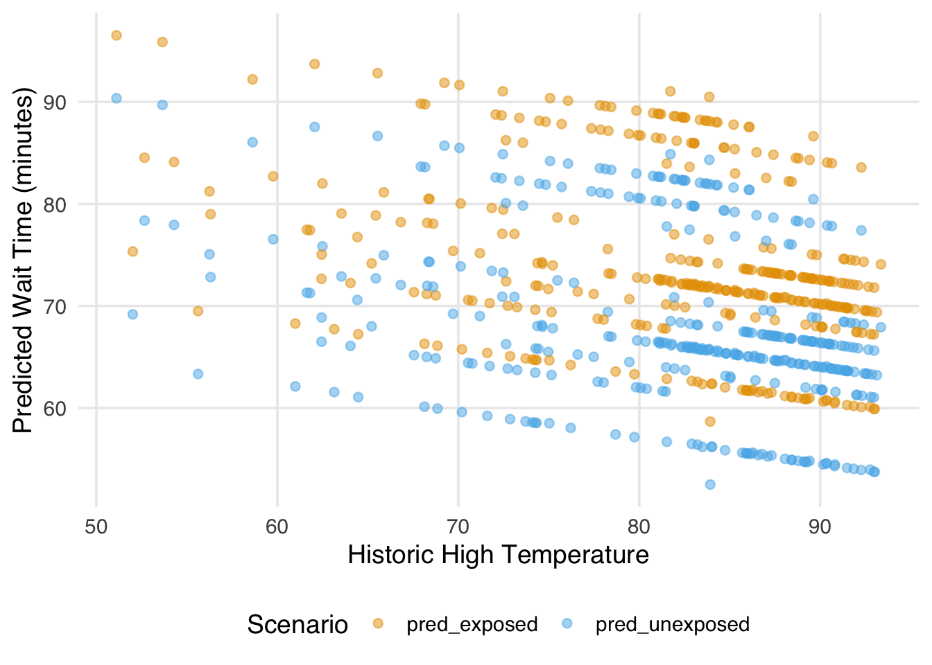
Each point represents a single park date predicted under the exposed and unexposed scenarios. Because we are using a linear model, the two sets of predictions are parallel (in other words, the gap between them is constant across the range of temperature). That gap, averaged across all park dates, is the estimated average treatment effect. Notice that we are not plugging in a single “representative” covariate value; we are generating predictions for every observation at their actual covariate values and then averaging. This is what it means to marginalize over the covariate distribution, and it is what distinguishes g-computation from simply extracting a coefficient from the outcome model.
The marginaleffects package makes some of these mechanics easy and help with uncertainty quantification. For example, rather than creating the separate counterfactual datasets, we can calculate the average treatment effect directly using the average_comparisons function.
library(marginaleffects)
ate <- avg_comparisons(
  gcomp_model,
  variables = "park_extra_magic_morning"
)

ate
 Estimate Std. Error    z Pr(>|z|)   S 2.5 % 97.5 %
     6.16       2.26 2.73  0.00636 7.3  1.74   10.6

Term: park_extra_magic_morning
Type: response
Comparison: 1 - 0
It is worth pausing here to connect back to the framework from Chapter 10. The estimand is the same whether we use IPW or an outcome model: \(E[Y(1)−Y(0)]\), the average treatment effect. What differs is the estimator, the recipe we use to get there. When we used IPW in Chapter 11, we reweighted the observed data to balance confounders across exposure groups. Above, with g-computation we fit the outcome model to directly estimate the potential outcomes under each exposure level and average their difference. Because these are different recipes for the same cake, we should not be surprised if they produce somewhat different estimates in practice. Each relies on its own modeling assumptions: IPW depends on a correctly specified propensity score model, while the outcome model depends on a correctly specified model for the outcome. When those models are wrong in different ways, the estimates will diverge.
When marginaleffects computes uncertainty estimates for quantities like average treatment effects, it relies on the delta method, a technique for approximating the variance of a transformation of estimated parameters. If you have a vector of coefficients \(\hat{\boldsymbol{\beta}}\) with known variance-covariance matrix \(\Sigma\), and you want the variance of some function \(g(\hat{\boldsymbol{\beta}})\) (like a predicted probability or a marginal effect), the delta method gives you:
\[ \text{Var}\left[g(\hat{\boldsymbol{\beta}})\right] \approx \nabla g(\hat{\boldsymbol{\beta}})^\top \, \Sigma \, \nabla g(\hat{\boldsymbol{\beta}}) \]
where \(\nabla g\) is the gradient of \(g\) with respect to \(\boldsymbol{\beta}\). marginaleffects handles this gradient computation automatically and propagates it through \(\Sigma\) to produce standard errors.
As we discussed in Chapter 10, the ATE is not the only causal estimand of interest. G-computation makes it straightforward to target different estimands by changing which covariate distribution we average over. For the ATE, we average predictions over the full observed sample. For the ATT, we average only over the covariate distribution of the exposed (in our case, days that actually had Extra Magic Morning hours). For the ATC, we average only over the unexposed. The outcome model is the same in all three cases; what changes is whose covariate values we use when generating predictions. We can target each of these estimands directly in avg_comparisons using the newdata argument:
# ATE: average over the full sample
avg_comparisons(
  gcomp_model,
  variables = "park_extra_magic_morning"
)
 Estimate Std. Error    z Pr(>|z|)   S 2.5 % 97.5 %
     6.16       2.26 2.73  0.00636 7.3  1.74   10.6

Term: park_extra_magic_morning
Type: response
Comparison: 1 - 0
# ATT: average over exposed observations only
avg_comparisons(
gcomp_model,
variables = "park_extra_magic_morning",
newdata = filter(seven_dwarfs_9, park_extra_magic_morning == 1)
)
 Estimate Std. Error    z Pr(>|z|)   S 2.5 % 97.5 %
     6.16       2.26 2.73  0.00636 7.3  1.74   10.6

Term: park_extra_magic_morning
Type: response
Comparison: 1 - 0
# ATC: average over unexposed observations only
avg_comparisons(
gcomp_model,
variables = "park_extra_magic_morning",
newdata = filter(seven_dwarfs_9, park_extra_magic_morning == 0)
)
 Estimate Std. Error    z Pr(>|z|)   S 2.5 % 97.5 %
     6.16       2.26 2.73  0.00636 7.3  1.74   10.6

Term: park_extra_magic_morning
Type: response
Comparison: 1 - 0
In this case, because our outcome model contains no interaction terms between the exposure and the covariates, the three estimates will be identical. A linear model without interactions assumes a constant treatment effect across all covariate values, so it does not matter whose covariate distribution we average over, we always recover the same gap. To see differences between the ATE, ATT, and ATC from g-computation, the outcome model needs to allow the effect of the exposure to vary with covariates, for example by including an interaction term like park_extra_magic_morning * park_ticket_season. Let’s refit our model to see these differences.
gcomp_model_int <- lm(
  wait_minutes_posted_avg ~
    park_extra_magic_morning +
    park_ticket_season +
    park_close +
    park_temperature_high +
    park_extra_magic_morning * park_ticket_season,
  data = seven_dwarfs_9
)

# ATE: average over the full sample
avg_comparisons(
  gcomp_model_int,
  variables = "park_extra_magic_morning"
)
 Estimate Std. Error    z Pr(>|z|)   S 2.5 % 97.5 %
     5.05       2.33 2.17   0.0302 5.1 0.484   9.62

Term: park_extra_magic_morning
Type: response
Comparison: 1 - 0
# ATT: average over exposed observations only
avg_comparisons(
gcomp_model_int,
variables = "park_extra_magic_morning",
newdata = filter(seven_dwarfs_9, park_extra_magic_morning == 1)
)
 Estimate Std. Error    z Pr(>|z|)   S 2.5 % 97.5 %
     6.34       2.23 2.84  0.00448 7.8  1.97   10.7

Term: park_extra_magic_morning
Type: response
Comparison: 1 - 0
# ATC: average over unexposed observations only
avg_comparisons(
gcomp_model_int,
variables = "park_extra_magic_morning",
newdata = filter(seven_dwarfs_9, park_extra_magic_morning == 0)
)
 Estimate Std. Error    z Pr(>|z|)   S 2.5 % 97.5 %
     4.79       2.38 2.01   0.0445 4.5 0.118   9.47

Term: park_extra_magic_morning
Type: response
Comparison: 1 - 0
Once at least one interaction has been specified, the three estimates can differ because the exposed and unexposed days tend to have different covariate distributions. The ATT asks what the effect was for the kinds of days that actually had Extra Magic Hours; the ATC asks what the effect would be for the kinds of days that did not. If the treatment effect were constant across all covariate values, the three estimates would coincide. When they differ, that divergence is itself informative about treatment effect heterogeneity across the population.
The same g-computation logic applies when the outcome is binary, but there are now three quantities of interest rather than one: the risk difference, the risk ratio, and the odds ratio (see Section 11.5). All three fall out of the same g-computation workflow; what changes is the function we apply to the predicted probabilities under each exposure.
Reusing the binary version of the wait-time outcome from Section 11.5, we fit a logistic g-computation model with the same confounders as the continuous version.
We can reuse the exposed and unexposed clones from earlier (the exposure hasn’t changed in this question, so the counterfactual scenarios are the same): predict the probability of the outcome under each, average the predictions, then combine the two means into whichever effect measure we want.
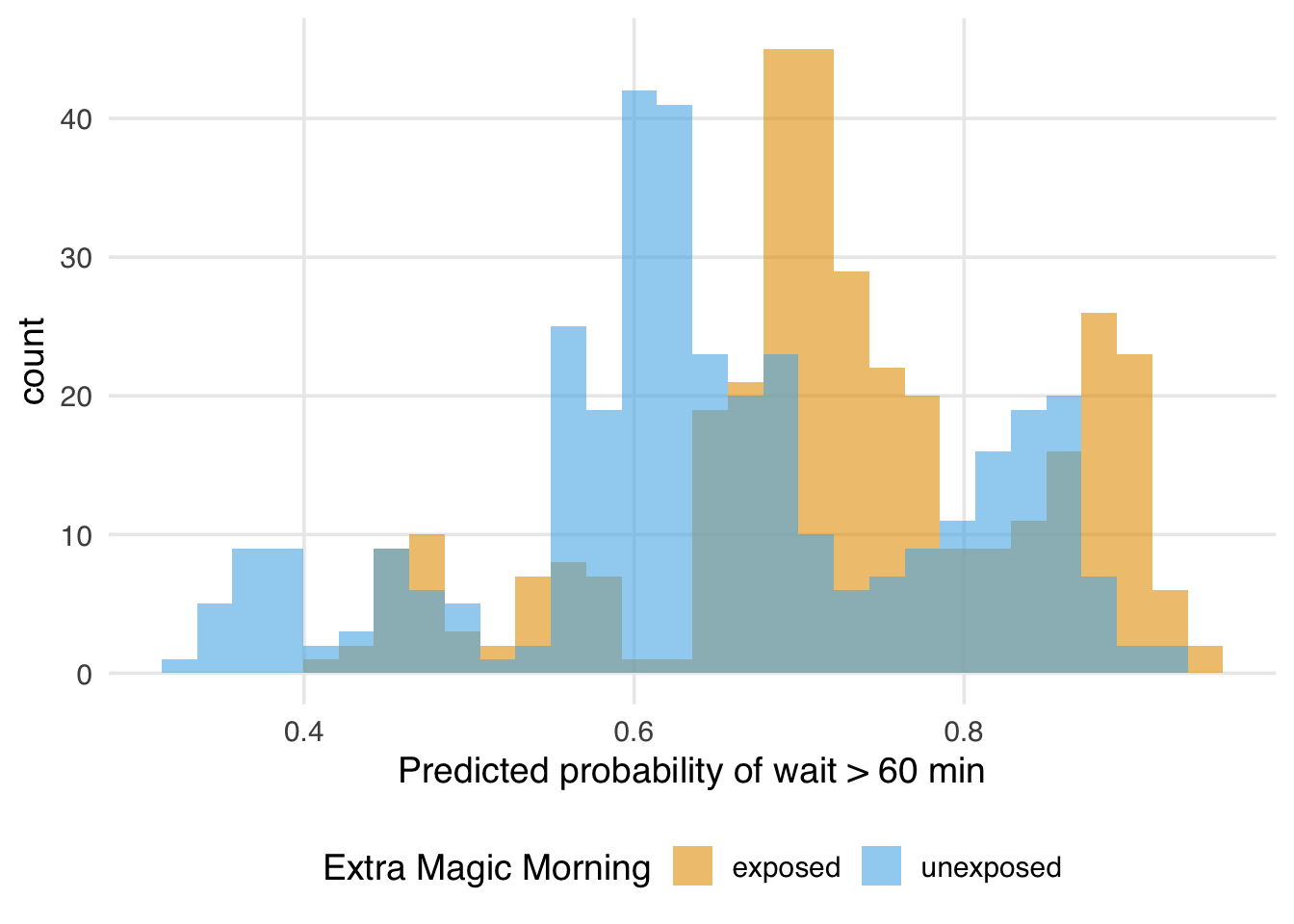
Plotting the predicted probabilities under each counterfactual shows what those marginal means are summarizing. The exposed distribution sits a little to the right of the unexposed one, which is exactly what a positive risk difference looks like at the level of individual predictions.
probs |>
  pivot_longer(
    everything(),
    names_to = "extra_magic_morning",
    values_to = "predicted_prob",
    names_prefix = "p_"
  ) |>
  ggplot(aes(x = predicted_prob, fill = extra_magic_morning)) +
  geom_histogram(alpha = 0.6, position = "identity", bins = 30) +
  labs(
    x = "Predicted probability of wait > 60 min",
    fill = "Extra Magic Morning"
  )
Now, let’s calculate each outcome measure.
probs |>
  summarize(
    p_exposed = mean(p_exposed),
    p_unexposed = mean(p_unexposed),
    rd = p_exposed - p_unexposed,
    rr = p_exposed / p_unexposed,
    or = (p_exposed / (1 - p_exposed)) /
      (p_unexposed / (1 - p_unexposed))
  )
# A tibble: 1 × 5
p_exposed p_unexposed rd rr or
<dbl> <dbl> <dbl> <dbl> <dbl>
1 0.728 0.651 0.0763 1.12 1.43This gets us point estimates but no uncertainty. We can, of course, bootstrap this, as with any technique we’ve discussed, but we’ll instead have marginaleffects compute the standard errors for us. avg_comparisons() produces the same numbers along with delta-method standard errors and confidence intervals, and selects the effect measure via its comparison argument. The default, "difference", gives the risk difference: the average difference between the predicted probability for the exposed and unexposed.
# Risk difference (ATE)
ate_rd <- avg_comparisons(
  gcomp_bin,
  variables = "park_extra_magic_morning"
)
ate_rd
 Estimate Std. Error   z Pr(>|z|)   S   2.5 % 97.5 %
   0.0763     0.0638 1.2    0.232 2.1 -0.0487  0.201

Term: park_extra_magic_morning
Type: response
Comparison: 1 - 0
For the risk ratio and odds ratio, we ask for the contrast on the log scale and back-transform with transform = exp. This is the standard approach for ratio measures: the delta-method confidence interval is built on the log scale, where it is symmetric, and then exponentiated to keep it bounded above zero. The corresponding shortcuts are "lnratioavg" and "lnoravg".
# Risk ratio (ATE)
ate_rr <- avg_comparisons(
  gcomp_bin,
  variables = "park_extra_magic_morning",
  comparison = "lnratioavg",
  transform = exp
)
ate_rr
 Estimate Pr(>|z|)   S 2.5 % 97.5 %
     1.12    0.216 2.2 0.937   1.33

Term: park_extra_magic_morning
Type: response
Comparison: ln(mean(1) / mean(0))
# Odds ratio (ATE)
ate_or <- avg_comparisons(
gcomp_bin,
variables = "park_extra_magic_morning",
comparison = "lnoravg",
transform = exp
)
ate_or
 Estimate Pr(>|z|)   S 2.5 % 97.5 %
     1.43    0.256 2.0 0.772   2.65

Term: park_extra_magic_morning
Type: response
Comparison: ln(odds(1) / odds(0))
These are the marginal ATE versions of each measure; the predictions are averaged over the full observed sample. Targeting the ATT or ATC works exactly as in Section 13.1.2: pass newdata to restrict the covariate distribution we average over.
# Risk difference (ATT)
avg_comparisons(
  gcomp_bin,
  variables = "park_extra_magic_morning",
  newdata = filter(seven_dwarfs_9, park_extra_magic_morning == 1)
)
 Estimate Std. Error    z Pr(>|z|)   S   2.5 % 97.5 %
    0.073     0.0615 1.19    0.236 2.1 -0.0476  0.194

Term: park_extra_magic_morning
Type: response
Comparison: 1 - 0
# Risk difference (ATC)
avg_comparisons(
gcomp_bin,
variables = "park_extra_magic_morning",
newdata = filter(seven_dwarfs_9, park_extra_magic_morning == 0)
)
 Estimate Std. Error   z Pr(>|z|)   S   2.5 % 97.5 %
    0.077     0.0643 1.2    0.231 2.1 -0.0489  0.203

Term: park_extra_magic_morning
Type: response
Comparison: 1 - 0
The same newdata argument can be combined with any of the comparison shortcuts above to target ATT or ATC versions of the risk ratio or odds ratio.
Following the advice in Section 11.5, we report the three effect measures together with the baseline probability of the outcome. The baseline here is the probability of an average wait over 60 minutes if no day had Extra Magic Mornings, which we can pull out of avg_predictions() by setting the exposure to 0 for everyone.
ate_baseline <- avg_predictions(
  gcomp_bin,
  variables = list(park_extra_magic_morning = 0)
)

summary_row <- function(x, label) {
  x |>
    as.data.frame() |>
    transmute(measure = label, estimate, conf.low, conf.high)
}

bind_rows(
  summary_row(ate_baseline, "Baseline probability"),
  summary_row(ate_rd, "Risk difference"),
  summary_row(ate_rr, "Risk ratio"),
  summary_row(ate_or, "Odds ratio")
)
measure estimate conf.low conf.high
1 Baseline probability 0.65147 0.59932 0.7036
2 Risk difference 0.07631 -0.04871 0.2013
3 Risk ratio 1.11714 0.93724 1.3316
4 Odds ratio 1.43033 0.77152 2.6517As we discussed in Section 11.5.2, odds ratios are non-collapsible: the conditional log-odds ratio reported in the glm() coefficient is generally not equal to the marginal odds ratio shown above, even when there is no confounding to adjust for. G-computation deliberately marginalizes over the covariate distribution. Because it’s a marginal OR, it’s also comparable to an unadjusted OR, whereas a conditional OR is not.
The same strategy applies when the exposure is continuous. For instance, imagine estimating how the actual wait time at 9am would change if the posted wait time at 8am were set to 60 minutes rather than 30 minutes. The procedure outlined above is identical, except that the exposure is set to the chosen numerical values for the counterfactual datasets.
Let’s start by arranging the data so that the actual wait time at 9 AM can be modeled using the posted wait time at 8 AM and the same confounders idenfied above.
We fit the outcome model the same way as for the binary exposure, as the outcome in both cases is continuous. Note now since we have a continuous exposure we can flexibly fit this, for example by using a natural spline.
To compare posted wait times of 60 and 30 minutes, two counterfactual datasets are constructed:
We then obtain predicted outcomes for each counterfactual dataset and then average these and take the difference:
pred_high <- fit_wait |> augment(newdata = high) |> select(pred_high = .fitted)
pred_low <- fit_wait |> augment(newdata = low) |> select(pred_low = .fitted)

bind_cols(pred_high, pred_low) |>
  summarize(
    mean_high = mean(pred_high),
    mean_low = mean(pred_low),
    difference = mean_high - mean_low
  )
# A tibble: 1 × 3
mean_high mean_low difference
<dbl> <dbl> <dbl>
1 29.8 40.7 -10.8The resulting difference estimates how much the actual wait time would change if posted wait time were set to these two specific values and all other variables remained as observed.
As above, we can also use the marginaleffects package along with the average_comparisons function:
comparison_30_60 <- avg_comparisons(
  fit_wait,
  variables = list(wait_minutes_posted_avg = c(30, 60))
)
comparison_30_60
 Estimate Std. Error     z Pr(>|z|)   S 2.5 % 97.5 %
    -10.8       8.13 -1.33    0.182 2.5 -26.8   5.09

Term: wait_minutes_posted_avg
Type: response
Comparison: 60 - 30G-computation handles poor overlap differently from IPW. When positivity is violated (or nearly so), IPW weights become extreme, destabilizing the estimate. G-computation sidesteps this by extrapolating from the outcome model into regions of the covariate space where one exposure group is rare. This can be an advantage if the model is correctly specified, but it also comes at a cost if not as it can mask potential problems.
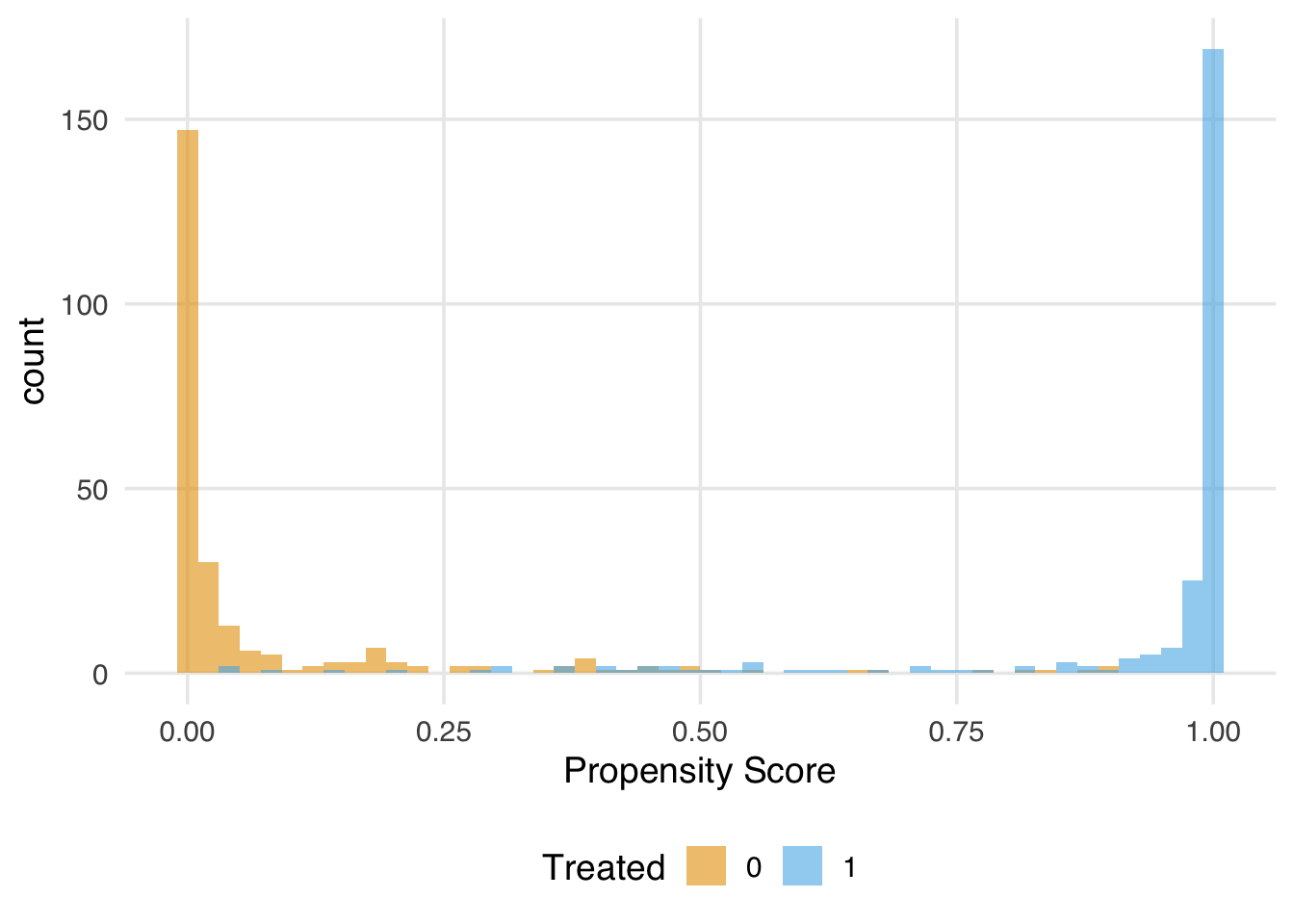
To see this, consider a toy dataset with poor overlap. Here, the confounder z strongly predicts treatment, so many observations have propensity scores near 0 or 1. The true outcome model includes a nonlinear (cubic) relationship between z and y.
The true ATE is 2. Let’s first examine the overlap.
library(propensity)
ps_model <- glm(x ~ z, data = sim_poor, family = binomial())
Warning: glm.fit: fitted probabilities numerically 0
or 1 occurredsim_poor <- sim_poor |>
mutate(
ps = predict(ps_model, type = "response"),
w_ate = wt_ate(ps, x, exposure_type = "binary", .focal_level = 1)
)
ggplot(sim_poor, aes(x = ps, fill = factor(x))) +
geom_histogram(bins = 50, alpha = 0.6, position = "identity") +
labs(
x = "Propensity Score",
fill = "Treated"
)
Now let’s see what happens to the IPW weights.
ggplot(sim_poor, aes(x = as.numeric(w_ate))) +
  geom_histogram(bins = 50) +
  labs(x = "ATE Weight")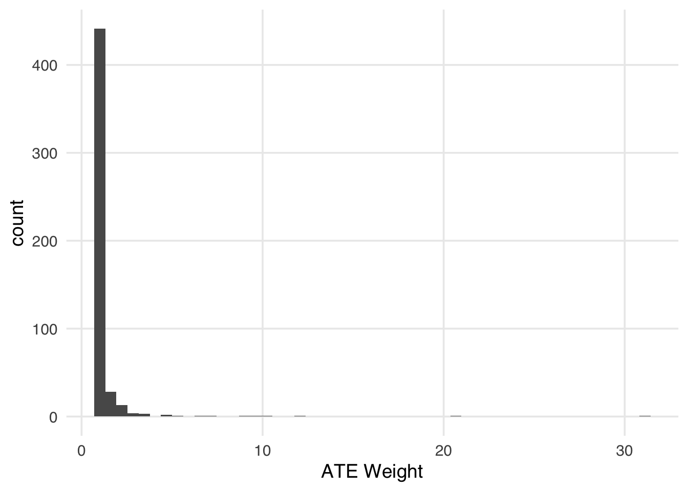
The IPW estimate is unstable as a result.
sim_poor |>
  summarize(
    ipw_ate = sum(y * x * w_ate) /
      sum(x * w_ate) -
      sum(y * (1 - x) * w_ate) / sum((1 - x) * w_ate)
  )
# A tibble: 1 × 1
ipw_ate
<dbl>
1 -1.24Now let’s try g-computation with a correctly specified outcome model, i.e., one that includes the cubic term for z.
gcomp_correct <- lm(y ~ x + z + I(z^3), data = sim_poor)

exposed_sim <- sim_poor |> mutate(x = 1)
unexposed_sim <- sim_poor |> mutate(x = 0)

bind_cols(
  augment(gcomp_correct, newdata = exposed_sim) |> select(pred_1 = .fitted),
  augment(gcomp_correct, newdata = unexposed_sim) |> select(pred_0 = .fitted)
) |>
  summarize(ate = mean(pred_1 - pred_0))
# A tibble: 1 × 1
ate
<dbl>
1 2.40With a correctly specified model, g-computation recovers an estimate close to the true ATE of 2, even under poor overlap. It achieves this by extrapolating the fitted outcome surface into regions of the covariate space where one group is rare, borrowing strength from the model rather than from observed counterparts.
However, this extrapolation only works if the outcome model is correctly specified. If we misspecify the model by omitting the cubic term, g-computation will extrapolate the wrong surface into exactly those regions where we have no data to detect the error.
gcomp_wrong <- lm(y ~ x + z, data = sim_poor)

bind_cols(
  augment(gcomp_wrong, newdata = exposed_sim) |> select(pred_1 = .fitted),
  augment(gcomp_wrong, newdata = unexposed_sim) |> select(pred_0 = .fitted)
) |>
  summarize(ate = mean(pred_1 - pred_0))
# A tibble: 1 × 1
ate
<dbl>
1 4.60The misspecified model produces a noticeably biased estimate. The bias is concentrated in the tails of the covariate distribution, exactly where overlap is poor and where we are relying most heavily on the model to fill in the gaps. We can see this by plotting the fitted outcome surfaces from the two models against the true cubic relationship.
z_seq <- tibble(z = seq(min(sim_poor$z), max(sim_poor$z), length.out = 200))

surfaces <- bind_rows(
  z_seq |>
    mutate(
      x = 1,
      correct = predict(gcomp_correct, newdata = mutate(z_seq, x = 1)),
      wrong = predict(gcomp_wrong, newdata = mutate(z_seq, x = 1)),
      group = "Treated"
    ),
  z_seq |>
    mutate(
      x = 0,
      correct = predict(gcomp_correct, newdata = mutate(z_seq, x = 0)),
      wrong = predict(gcomp_wrong, newdata = mutate(z_seq, x = 0)),
      group = "Untreated"
    )
)

ggplot() +
  geom_point(
    data = sim_poor,
    aes(x = z, y = y, color = factor(x)),
    alpha = 0.3,
    size = 0.8
  ) +
  geom_line(
    data = surfaces,
    aes(x = z, y = correct, color = group),
    linewidth = 1
  ) +
  geom_line(
    data = surfaces,
    aes(x = z, y = wrong, color = group),
    linewidth = 1,
    linetype = "dashed"
  ) +
  labs(
    x = "z",
    y = "y",
    color = "Group",
    caption = "Solid lines: correctly specified model. Dashed lines: misspecified model."
  )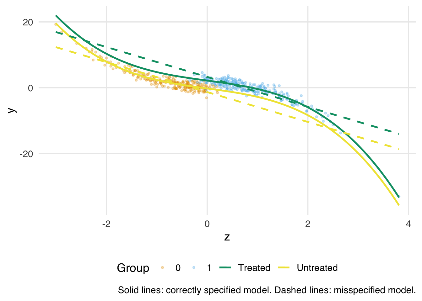
The takeaway is that g-computation and IPW face a fundamental tradeoff when overlap is poor. IPW makes its reliance on overlap explicit (i.e., the weights blow up and the analyst is forced to confront the problem). G-computation absorbs the problem silently, producing a stable estimate that may nonetheless be wrong. Neither method can conjure causal information that is not in the data; g-computation simply moves the assumption from the propensity score model to the outcome model. When overlap is poor, getting the functional form of the outcome model right in the tails matters, and it is precisely in those regions that we have the least data to check it.