Work-in-progress 🚧
You are reading the work-in-progress first edition of Causal Inference in R. This chapter is actively undergoing work and may be restructured or changed. It may also be incomplete.
You are reading the work-in-progress first edition of Causal Inference in R. This chapter is actively undergoing work and may be restructured or changed. It may also be incomplete.
As discussed in Chapter 10, causal estimands such as the ATE, ATT, and ATC are all defined as expectations of the same unit-level contrast, \((Y(1)-Y(0))\), but taken over different covariate distributions. This distinction becomes meaningful only when the individual treatment effect varies across units.
Note here we denote \(\mathbf{Z}\) in bold. This is to indicate that this represents several covariates (in practice, all of the confounders), rather than a single variable
As defined in Section 3.1, \(Y(1)\) and \(Y(0)\) denote potential outcomes under exposure \((X=1)\) and control \((X=0)\). \(\mathbf{Z}\) is a vector of pre-treatment covariates. The individual treatment effect can be written as
\[ \tau(Z)=Y(1)-Y(0). \]
Heterogeneous treatment effects arise when \(\tau(Z)\) is not constant in \(Z\). In that case, we see the various estimands defined in Chapter 10, for example
\[ \text{ATE}=E[\tau(Z)], \quad \text{ATT}=E[\tau(Z)\mid X=1], \quad \text{ATC}=E[\tau(Z)\mid X=0]. \]
The above are different averages of the same function \(\tau(Z)\). Any difference between them is driven by two things: 1. variation in treatment effects across covariate profiles, and 2. differences in the distribution of those covariate profiles across treated and untreated units.
Suppose we fit a simple regression model to understand the relationship between an exposure and outcome. In other words, we model the conditional mean of the observed outcome \(Y\) as a function of treatment \(X\) and confounders \(\mathbf{Z}\).
\[ E[Y\mid X,Z]=\beta_0+\beta_1X+\boldsymbol\beta^\top \textbf{Z} \] Under this specification,
\[ E[Y\mid X=1,\mathbf{Z}]-E[Y\mid X=0,\mathbf{Z}]=\beta_1. \]
This means the treatment effect is assumed to be the same for every unit, regardless of covariate values. In other words, after adjusting for \(\mathbf{Z}\), the model assumes the effect of treatment does not vary across the population.
That can be a strong assumption. In many settings, treatment effects may differ across subgroups. To allow for this possibility, suppose one variable in the confounder set \(\mathbf{Z}\) modifies the treatment effect (let’s call this \(Z_1\)). We can include an interaction between treatment and that covariate:
\[ E[Y \mid X,\mathbf{Z}] = \beta_0 + \beta_1 X + \beta_2 Z_1 + \beta_3(X \times Z_1) + \boldsymbol{\beta}_4^{\top}\mathbf{W}, \]
where \(\mathbf{W}\) contains the remaining covariates in \(\mathbf{Z}\) excluding \(Z_1\). Then the conditional treatment effect becomes
\[ \tau(Z_1)= E[Y \mid X=1,\mathbf{Z}] - E[Y \mid X=0,\mathbf{Z}] =\beta_1 + \beta_3 Z_1. \]
Now the treatment effect depends on \(Z_1\). If \(\beta_3=0\), the treatment effect is constant, otherwise the treatment effect changes across values of \(Z_1\).
This is one way regression models represent heterogeneous treatment effects. The interaction term formalizes the claim that the effect of treatment differs across levels of a covariate.
An equivalent way to represent the same idea is to fit separate regression models within strata of \(Z_1\) (or if \(Z_1\) is categorical, fitting the model within each category). Separate models allow the treatment coefficient to differ across groups. The interaction model is often preferred because it estimates those subgroup-specific effects within a single unified framework while using all available data simultaneously.
G-computation makes the link between conditional effects and marginal estimands explicit. After fitting an outcome model, we generate two predictions for each unit:
\[ \hat Y_i(1)=\widehat{E}[Y\mid X=1,Z_i], \quad \hat Y_i(0)=\widehat{E}[Y\mid X=0,Z_i]. \]
This gives a unit-level estimated treatment effect:
\[ \hat\tau_i=\hat Y_i(1)-\hat Y_i(0). \]
When interactions are present, \(\hat\tau_i\) varies across units because it depends on \(Z_i\). The ATE is then
\[ \widehat{\text{ATE}}=\frac{1}{n}\sum_{i=1}^n \hat\tau_i. \] The ATT and ATC are obtained by averaging over treated or untreated subsets instead. Let’s return to the example from Section 13.1.2. Once again, we are interested in understanding the relationship between whether a particular day offers Extra Magic Morning hours and the average posted wait time at the Seven Dwarfs Mine Train ride between 9 and 10am. Here, we allow the effect of Extra Magic Morning to vary by ticket season through an interaction term. Once treatment effects are allowed to differ across covariate profiles, g-computation averages different unit-level effects over different target populations, and the ATE, ATT, and ATC need not coincide.
library(tidyverse)
library(broom)
library(touringplans)
library(marginaleffects)

seven_dwarfs_9 <- seven_dwarfs_train_2018 |>
  filter(wait_hour == 9)

gcomp_model_int <- lm(
  wait_minutes_posted_avg ~
    park_extra_magic_morning +
    park_ticket_season +
    park_close +
    park_temperature_high +
    park_extra_magic_morning * park_ticket_season,
  data = seven_dwarfs_9
)

# ATE: average over the full sample
avg_comparisons(
  gcomp_model_int,
  variables = "park_extra_magic_morning"
)
 Estimate Std. Error    z Pr(>|z|)   S 2.5 % 97.5 %
     5.05       2.33 2.17   0.0302 5.1 0.484   9.62

Term: park_extra_magic_morning
Type: response
Comparison: 1 - 0
# ATT: average over exposed observations only
avg_comparisons(
gcomp_model_int,
variables = "park_extra_magic_morning",
newdata = filter(seven_dwarfs_9, park_extra_magic_morning == 1)
)
 Estimate Std. Error    z Pr(>|z|)   S 2.5 % 97.5 %
     6.34       2.23 2.84  0.00448 7.8  1.97   10.7

Term: park_extra_magic_morning
Type: response
Comparison: 1 - 0
# ATC: average over unexposed observations only
avg_comparisons(
gcomp_model_int,
variables = "park_extra_magic_morning",
newdata = filter(seven_dwarfs_9, park_extra_magic_morning == 0)
)
 Estimate Std. Error    z Pr(>|z|)   S 2.5 % 97.5 %
     4.79       2.38 2.01   0.0445 4.5 0.118   9.47

Term: park_extra_magic_morning
Type: response
Comparison: 1 - 0
Once interaction is introduced, these estimands can differ because they average the same heterogeneous response surface over different covariate distributions. Because g-computation focuses on modeling the outcome we must specify every interaction we think exists in order to accurately estimate treatment effect heterogeneity.
Inverse probability weighting targets the same estimands through a different mechanism. Rather than modeling \(E[Y\mid X,\mathbf{Z}]\) directly, IPW reweights the data so treatment assignment is independent of \(Z\).
Unlike g-computation, IPW does not require us to specify an explicit regression model for the outcome surface. The weighting scheme determines which covariate distribution is used to average those heterogeneous unit-level effects. Just as with g-computation, ATE, ATT, and ATC can differ when treatment effects vary across covariate profiles, but we didn’t need to specify the interaction terms explicitly to see these differences. IPW captures heterogeneity implicitly through the weighting and averaging target, not by estimating subgroup-specific treatment effects.
Let’s look at the same example as above. As in Chapter 11, we first estimate the propensity score, the probability of receiving Extra Magic Morning conditional on observed covariates:
We then pull the propensity scores from this model and estimate the weights according to the estimand of interest.
library(propensity)
seven_dwarfs_9_with_ps <- propensity_model |>
  augment(type.predict = "response", data = seven_dwarfs_9)

seven_dwarfs_9_with_wt <- seven_dwarfs_9_with_ps |>
  mutate(
    w_ate = wt_ate(.fitted, park_extra_magic_morning),
    w_att = wt_att(.fitted, park_extra_magic_morning),
    w_atc = wt_atc(.fitted, park_extra_magic_morning)
  )
Finally we get our estimates by fitting the weighted outcome models:
# ATE
lm(
  wait_minutes_posted_avg ~ park_extra_magic_morning,
  data = seven_dwarfs_9_with_wt,
  weights = w_ate
) |>
  tidy()
# A tibble: 2 × 5
term estimate std.error statistic p.value
<chr> <dbl> <dbl> <dbl> <dbl>
1 (Intercept) 68.1 1.38 49.4 2.60e-160
2 park_extra_ma… 6.20 1.95 3.19 1.57e- 3# ATT
lm(
wait_minutes_posted_avg ~ park_extra_magic_morning,
data = seven_dwarfs_9_with_wt,
weights = w_att
) |>
tidy()# A tibble: 2 × 5
term estimate std.error statistic p.value
<chr> <dbl> <dbl> <dbl> <dbl>
1 (Intercept) 68.7 1.45 47.3 1.69e-154
2 park_extra_ma… 6.23 2.05 3.03 2.62e- 3# ATC
lm(
wait_minutes_posted_avg ~ park_extra_magic_morning,
data = seven_dwarfs_9_with_wt,
weights = w_atc
) |>
tidy()# A tibble: 2 × 5
term estimate std.error statistic p.value
<chr> <dbl> <dbl> <dbl> <dbl>
1 (Intercept) 67.9 1.36 49.9 1.28e-161
2 park_extra_ma… 6.19 1.92 3.22 1.39e- 3Up to this point, we have used interaction terms in regression models to represent heterogeneous treatment effects: the effect of the exposure varies across levels of a covariate \(\mathbf{Z}\). That is often pracitioners mean when they ask whether an effect “differs by subgroup.” It can be useful to distinguish two related but different ideas: effect modification and interaction (Weinberg 2007; VanderWeele 2009; Nilsson et al. 2020; Hernán and Robins 2021). These terms are often used interchangeably, but they answer different causal questions. Effect modification asks whether the causal effect of treatment \(X\) on outcome \(Y\) differs across levels of some pre-treatment variable \(Z\). In our notation, this is the question:
\[ E[Y(1)-Y(0)\mid Z=z_1] \neq E[Y(1)-Y(0)\mid Z=z_0]. \]
Here, \(Z\) is used to define subgroups. We are interested in how the effect of \(X\) changes across observed strata of \(Z\), not in intervening on \(Z\) itself.
For the Seven Dwarfs example, \(Z\) might be park_ticket_season. Then the question is whether Extra Magic Morning changes posted wait time differently during peak season versus off-season.
Causal interaction, by contrast, treats both variables as exposures of causal interest. Instead of asking whether the effect of \(X\) varies across strata of \(Z\), it asks whether the joint effect of changing both \(X\) and \(Z\) differs from what would be expected based on their separate effects.
Formally, causal interaction compares counterfactual contrasts such as
\[ E[Y(x_1,z_1)-Y(x_0,z_1)] \neq E[Y(x_1,z_0)-Y(x_0,z_0)]. \]
This may look similar to effect modification, but the interpretation is different. In effect modification, \(Z\) is a subgroup-defining characteristic. In causal interaction, \(Z\) is itself something we conceptually intervene on. That distinction matters because some variables are natural subgroup indicators but not plausible intervention targets. For example, season, age group, or baseline risk category may be useful effect modifiers, even though we would not think of “assigning” people to them in the same way we assign an exposure.
In the Seven Dwarfs setting, asking whether the effect of Extra Magic Morning differs by park_ticket_season is naturally an effect-modification question: does the policy work differently in busy versus less busy periods? That is different from asking about the joint causal effect of changing both Extra Magic Morning access and ticket season itself.
In practice, many regression models with interaction terms are used to study effect modification rather than interaction in the stricter causal sense. The same algebraic model can serve either purpose, but interpretation depends on the underlying question.
For most policy and applied settings, the subgroup question is the relevant one: who benefits more, who benefits less, and how does the average effect depend on population composition? That is why heterogeneous treatment effects and effect modification are central to causal inference, transportability, and targeting interventions.
As noted in Chapter 4, conventional DAGs don’t inherently represent interaction or effect modification, though some proposals exist to include these features. Here we demonstrate three approaches using a simple example where \(X\) (exposure) and \(Q\) (another exposure) may interact in their effect on Y (outcome), with \(Z\) as a confounder.
The standard approach is to draw a conventional DAG without explicitly representing interactions.
conventional_dag <- dagify(
  X ~ Z,
  Q ~ Z,
  Y ~ X + Q + Z,
  coords = time_ordered_coords(
    list(
      c("Z"),
      c("X", "Q"),
      "Y"
    )
  ),
  exposure = "X",
  outcome = "Y",
  labels = c(
    X = "X",
    Y = "Y",
    Z = "Z",
    Q = "Q"
  )
)

ggdag(conventional_dag) +
  theme_dag()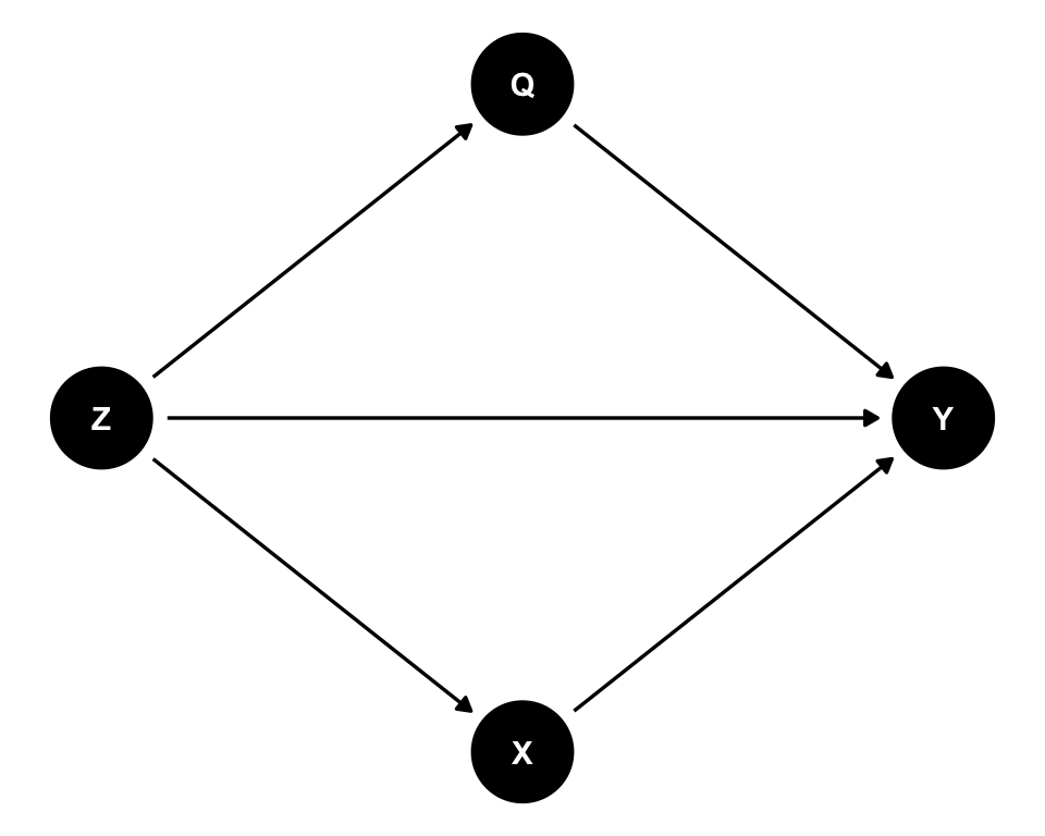
HEAD This DAG shows that X, Q, and Z all affect Y, but it doesn’t explicitly indicate whether X and Q interact. The interaction, if present, would be implicit in the functional form of how X and Q jointly affect Y in a statistical model.
Attia, Holliday, and Oldmeadow (2022) proposed representing interactions explicitly by adding an interaction node (like XxQ) to conventional DAGs.
explicit_interaction_dag <- dagify(
  X ~ Z,
  Q ~ Z,
  Y ~ X + Q + Z + XxQ,
  XxQ ~ X + Q,
  coords = time_ordered_coords(
    list(
      c("Z"),
      c("X", "Q"),
      "XxQ",
      "Y"
    )
  ),
  exposure = "X",
  outcome = "Y",
  labels = c(
    X = "X",
    Y = "Y",
    Z = "Z",
    Q = "Q",
    XxQ = "X × Q\ninteraction"
  )
)

ggdag(explicit_interaction_dag) +
  theme_dag()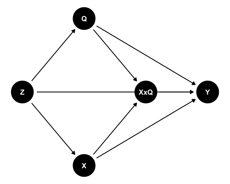
This approach makes the interaction explicit: arrows from X and Q point to XxQ, and XxQ points to Y. This can help identify appropriate adjustment sets for estimating interaction effects (Attia, Holliday, and Oldmeadow 2022). The DAG maintains conventional DAG conventions and can be drawn using standard DAG software.
Nilsson et al. (2020) proposed a different approach: interaction DAGs (IDAGs) that replace the outcome node with a node representing a causal effect measure.
# Note: IDAGs represent causal effects rather than outcomes
# This is a simplified representation - full IDAGs would show the effect node
# For demonstration, we show a conceptual version
idag_dag <- dagify(
  X ~ Z,
  Q ~ Z,
  Effect ~ X + Q + Z,
  coords = time_ordered_coords(
    list(
      c("Z"),
      c("X", "Q"),
      "Effect"
    )
  ),
  exposure = "X",
  outcome = "Effect",
  labels = c(
    X = "X",
    Effect = "Causal\neffect",
    Z = "Z",
    Q = "Q"
  )
)

ggdag(idag_dag) +
  theme_dag()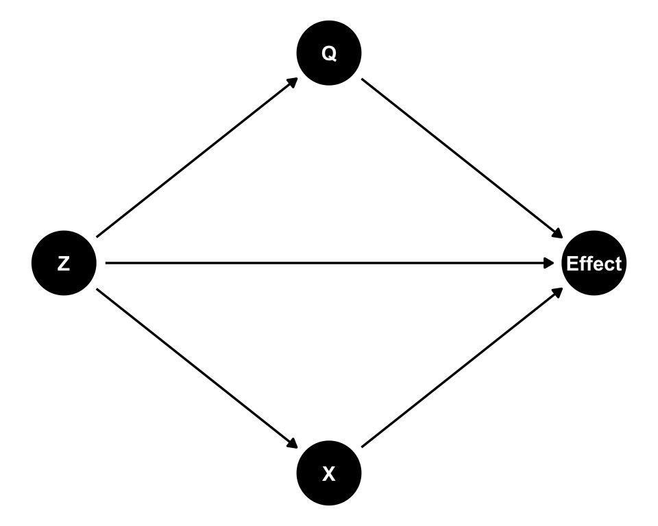
In IDAGs, instead of depicting how different variables influence the outcome, the DAG depicts how different variables influence the size of a chosen effect measure (Nilsson et al. 2020). This framework separates interactions from main effects, typically requiring separate DAGs for main effects and interactions. IDAGs preserve usual DAG conventions for reading and interpreting causal relationships.
Each approach has advantages:
The choice depends on your goals. If you want to make interactions explicit within a single diagram, the explicit interaction node approach may be most practical. If you’re conducting a detailed analysis of interaction mechanisms, IDAGs provide a more formal framework. For most purposes, conventional DAGs suffice, with interactions handled in the statistical modeling stage.