4 Target trials and standard methods
4.1 Randomized trials
A randomized trial is one where the exposure (cause) of interest is randomly assigned.
In this book, we refer to analyses where the exposure is randomly assigned as a randomized trial, sometimes this is called an A/B test.
Why does randomization help? Looking at our assumptions in Section 3.3, randomized trials solve the well defined exposure portion of consistency by default – the exposure is exactly what is randomized. Likewise for positivity; if we have randomly assigned folks to either the exposed or unexposed groups, we know the probability of assignment (and we know it is not exactly 0 or 1). Randomization alone does not solve the interference portion of consistency (for example, if we randomize some people to receive a vaccine for a communicable disease, their receiving it could lower the chance of those around them contracting the infectious disease because it changes the probability of exposure). Ideal randomized trials resolves the issue of exchangeability because the exposed and unexposed populations (in the limit) are inherently the same since their exposure status was determined by a random process (not by any factors that might make them different from each other). Great! In reality, we often see this assumption violated by issues such as drop out or non-adherence in randomized trials. If there is differential drop out between exposure groups (for example, if participants randomly assigned to the treatment are more likely to drop out of a study, and thus we don’t observe their outcome), then the observed exposure groups are no longer exchangeable. Therefore, in Table 4.1 we have two columns, one for the ideal randomized trial (where adherence is assumed to be perfect and no participants drop out) and one for realistic randomized trials where this may not be so.
| Assumption | Ideal Randomized Trial | Realistic Randomized Trial | Observational Study |
|---|---|---|---|
| Consistency (Well defined exposure) | 😄 | 😄 | 🤷 |
| Consistency (No interference) | 🤷 | 🤷 | 🤷 |
| Positivity | 😄 | 😄 | 🤷 |
| Exchangeability | 😄 | 🤷 | 🤷 |
When designing a study, the first step is asking an appropriate causal question. We then can map this question to a protocol, consisting of the following seven elements, as defined by Hernán and Robins (2016):
- Eligibility criteria
- Exposure definition
- Assignment procedures
- Follow-up period
- Outcome definition
- Causal contrast of interest
- Analysis plan
In Table 4.2 we map each of these elements to the corresponding assumption that it can address. For example, exchangeability can be addressed by the eligibility criteria (we can restrict our study to only participants for whom exposure assignment is exchangeable), assignment procedure (we could use random exposure assignment to ensure exchangeability), follow-up period (we can be sure to choose an appropriate start time for our follow-up period to ensure that we are not inducing bias – we’ll think more about this in a future chapter), and/or the analysis plan (we can adjust for any factors that would cause those in different exposure groups to lack exchangeability).
| Assumption | Eligibility Criteria | Exposure Definition | Assignment Procedures | Follow-up Period | Outcome Definition | Causal contrast | Analysis Plan |
|---|---|---|---|---|---|---|---|
| Consistency (Well defined exposure) | ✔️ | ✔️ | |||||
| Consistency (No interference) | ✔️ | ✔️ | ✔️ | ✔️ | |||
| Positivity | ✔️ | ✔️ | ✔️ | ||||
| Exchangeability | ✔️ | ✔️ | ✔️ | ✔️ |
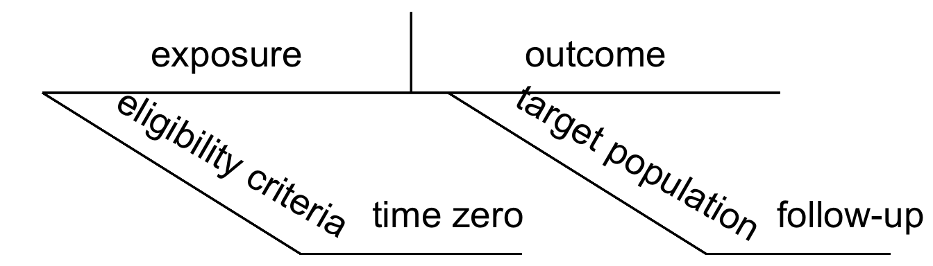
Recall our diagrams from Section 1.3 (Figure 4.1); several of these protocol elements can be mapped to these diagrams when we are attempting to define our causal question.
4.2 Target Trials
There are many reasons why randomization may not be possible. For example, it might not be ethical to randomly assign people to a particular exposure, there may not be funding available to run a randomized trial, or there might not be enough time to conduct a full trial. In these situations, we rely on observational data to help us answer causal questions by implementing a target trial.
A target trial answers: What experiment would you design if you could? Specifying a target trial is nearly identical to the process we described for a randomized trial. We define eligibility, exposure, follow-up period, outcome, estimate of interest, and the analysis plan. The key difference with the target trial in the observational setting, of course, is that we cannot assign exposure. The analysis planning and execution step of the target trial is the most technically involved and a core focus of this book; e.g. using DAGs to ensure that we have measured and are controlling for the right set of confounders, composing statistical programs that invoke an appropriate adjustment method such as IP weighting, and conducting sensitivity analyses to assess how sensitive our conclusions are to unmeasured confounding or misspecification.
4.3 Causal inference with group_by() and summarize()
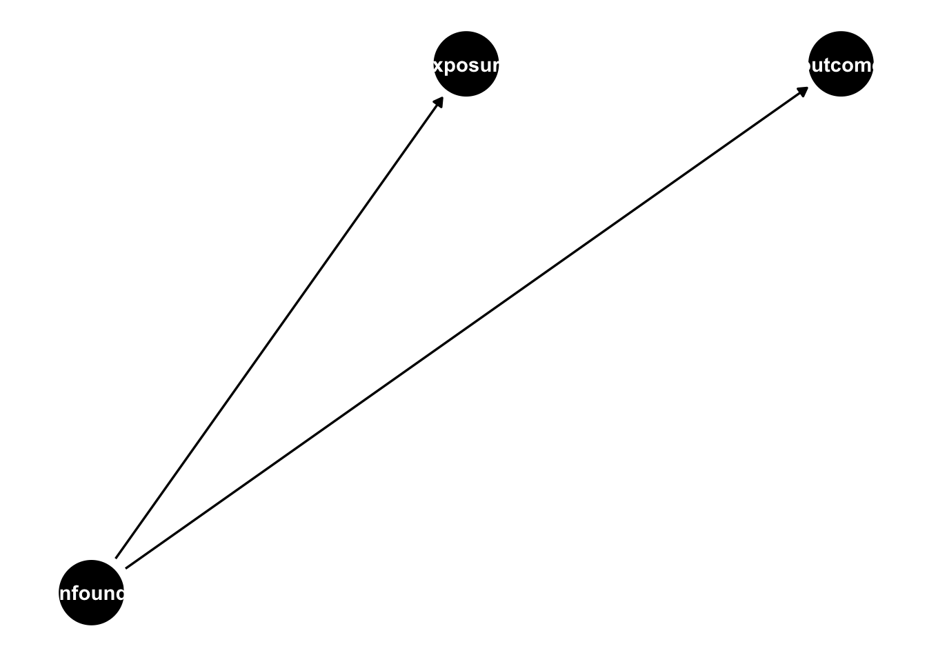
Let’s suppose we are trying to estimate a causal effect of an exposure on an outcome, but the exposure is not randomized, in fact, there is a common cause of the exposure and outcome, making the exposed and unexposed groups not exchangeable without adjustment (violating the fourth assumption in Section 3.3).
A confounder is a common cause of exposure and outcome.
4.3.1 One binary confounder
Let’s suppose this confounder is binary, see the simulation below:
set.seed(1)
n <- 10000
sim <- tibble(
  # generate the confounder from a binomial distribution
  # with a probability 0.5 for being in either group
  confounder = rbinom(n, 1, 0.5),
  # make the probability of exposure dependent on the
  # confounder value
  p_exposure = case_when(
    confounder == 1 ~ 0.75,
    confounder == 0 ~ 0.25
  ),
  # generate the exposure from a binomial distribution
  # with the probability of exposure dependent on the confounder
  exposure = rbinom(n, 1, p_exposure),
  # generate the "true" average treatment effect of 0
  # to do this, we are going to generate the potential outcomes, first
  # the potential outcome if exposure = 0
  # (notice exposure is not in the equation below, only the confounder)
  # we use rnorm(n) to add the random error term that is normally
  # distributed with a mean of 0 and a standard deviation of 1
  y0 = confounder + rnorm(n),
  # because the true effect is 0, the potential outcome if exposure = 1
  # is identical
  y1 = y0,
  # now, in practice we will only see one of these, outcome is what is
  # observed
  outcome = (1 - exposure) * y0 + exposure * y1,
  observed_potential_outcome = case_when(
    exposure == 0 ~ "y0",
    exposure == 1 ~ "y1"
  )
)
Here we have one binary confounder, the probability that confounder = 1 is 0.5. The probability of the being exposed is 0.75 for those for whom confounder = 1 0.25 for those for whom confounder = 0. There is no effect of the exposure on the outcome (the true causal effect is 0); the outcome effect is fully dependent on the confounder.
In this simulation we generate the potential outcomes to drive home our assumptions; many of our simulations in this book will skip this step. Let’s look at this generated data frame.
sim |>
  select(confounder, exposure, outcome, observed_potential_outcome)
# A tibble: 10,000 × 4
confounder exposure outcome observed_potential_out…¹
<int> <int> <dbl> <chr>
1 0 0 -0.804 y0
2 0 0 -1.06 y0
3 1 1 -0.0354 y1
4 1 1 -0.186 y1
5 0 0 -0.500 y0
6 1 1 0.475 y1
7 1 0 0.698 y0
8 1 0 1.47 y0
9 1 0 0.752 y0
10 0 0 1.26 y0
# ℹ 9,990 more rows
# ℹ abbreviated name: ¹observed_potential_outcomeGreat! Let’s begin by proving to ourselves that this violates the exchangeability assumption. Recall from Section 3.3:
Exchangeability: We assume that within levels of relevant variables (confounders), exposed and unexposed subjects have an equal likelihood of experiencing any outcome prior to exposure; i.e. the exposed and unexposed subjects are exchangeable. This assumption is sometimes referred to as no unmeasured confounding, though exchangeability implies more than that, such as no selection bias and that confounder relationships are appropriately specified. We will further define exchangeability through the lens of DAGs in the next chapter.
Now, let’s try to estimate the effect of the exposure on the outcome assuming the two exposed groups are exchangeable.
sim |>
  group_by(exposure) |>
  summarise(avg_outcome = mean(outcome))
# A tibble: 2 × 2
exposure avg_outcome
<int> <dbl>
1 0 0.228
2 1 0.756The average outcome among the exposed is 0.76 and among the unexposed 0.23, yielding an average effect of the exposure of 0.76-0.23=0.53. Let’s do a little R work to get there.
sim |>
  group_by(exposure) |>
  summarise(avg_outcome = mean(outcome)) |>
  pivot_wider(
    names_from = exposure,
    values_from = avg_outcome,
    names_prefix = "x_"
  ) |>
  summarise(estimate = x_1 - x_0)
# A tibble: 1 × 1
estimate
<dbl>
1 0.528Ok, so assuming the exposure groups are exchangeable (and assuming the rest of the assumptions from Section 3.3 hold), we estimate the effect of the exposure on the outcome to be 0.53. We know the exchangeability assumption is violated based on how we simulated the data. How can we estimate an unbiased effect? The easiest way to do so is to estimate the effect within each confounder class. This will work because folks with the same value of the confounder have an equal probability of exposure. Instead of just grouping by the exposure, let’s group by the confounder as well:
sim |>
  group_by(confounder, exposure) |>
  summarise(avg_outcome = mean(outcome))
# A tibble: 4 × 3
# Groups: confounder [2]
confounder exposure avg_outcome
<int> <int> <dbl>
1 0 0 -0.0185
2 0 1 0.00954
3 1 0 0.994
4 1 1 1.01 We can now calculate the average effect within each confounder class as well as the overall causal effect.
## Average effect within each confounder class
sim |>
  group_by(confounder, exposure) |>
  summarise(avg_outcome = mean(outcome)) |>
  pivot_wider(
    names_from = exposure,
    values_from = avg_outcome,
    names_prefix = "x_"
  ) |>
  summarise(estimate = x_1 - x_0)
# A tibble: 2 × 2
confounder estimate
<int> <dbl>
1 0 0.0280
2 1 0.0122## Overall average effect
sim |>
group_by(confounder, exposure) |>
summarise(avg_outcome = mean(outcome)) |>
pivot_wider(
names_from = exposure,
values_from = avg_outcome,
names_prefix = "x_"
) |>
summarise(estimate = x_1 - x_0) |>
summarise(mean(estimate)) # note, we would need to weight this if the confounder groups were not equal sized# A tibble: 1 × 1
`mean(estimate)`
<dbl>
1 0.0201Great! Now our estimate is much closer to the true value (0).
4.3.2 Two binary confounders
Let’s extend this to two binary confounders. The simulation below now has two binary confounders. The true causal effect of the exposure on the outcome is still 0.
set.seed(1)
n <- 10000
sim2 <- tibble(
  confounder_1 = rbinom(n, 1, 0.5),
  confounder_2 = rbinom(n, 1, 0.5),
  p_exposure = case_when(
    confounder_1 == 1 & confounder_2 == 1 ~ 0.75,
    confounder_1 == 0 & confounder_2 == 1 ~ 0.9,
    confounder_1 == 1 & confounder_2 == 0 ~ 0.2,
    confounder_1 == 0 & confounder_2 == 0 ~ 0.1,
  ),
  exposure = rbinom(n, 1, p_exposure),
  outcome = confounder_1 + confounder_2 + rnorm(n)
)
Now we are going to group by both confounders and estimate the causal effect within each stratum.
sim2 |>
  group_by(confounder_1, confounder_2, exposure) |>
  summarise(avg_y = mean(outcome)) |>
  pivot_wider(
    names_from = exposure,
    values_from = avg_y,
    names_prefix = "x_"
  ) |>
  summarise(estimate = x_1 - x_0)
# A tibble: 4 × 3
# Groups: confounder_1 [2]
confounder_1 confounder_2 estimate
<int> <int> <dbl>
1 0 0 -0.122
2 0 1 0.0493
3 1 0 0.0263
4 1 1 0.0226We can also estimate the overall causal effect:
sim2 |>
  group_by(confounder_1, confounder_2, exposure) |>
  summarise(avg_outcome = mean(outcome)) |>
  pivot_wider(
    names_from = exposure,
    values_from = avg_outcome,
    names_prefix = "x_"
  ) |>
  summarise(estimate = x_1 - x_0, .groups = "drop") |>
  summarise(mean(estimate))
# A tibble: 1 × 1
`mean(estimate)`
<dbl>
1 -0.005944.3.3 Continuous confounder
So far our strategy has been to estimate the causal effect within strata where the individuals are exchangeable. How could we extend this to a continuous confounder? Let’s create another simulation:
sim3# A tibble: 10,000 × 4
confounder p_exposure exposure outcome
<dbl> <dbl> <int> <dbl>
1 -0.626 0.348 0 -0.840
2 0.184 0.546 1 0.0769
3 -0.836 0.302 0 -1.30
4 1.60 0.831 1 0.911
5 0.330 0.582 1 -0.461
6 -0.820 0.306 0 -1.16
7 0.487 0.620 1 -0.780
8 0.738 0.677 1 -0.656
9 0.576 0.640 1 0.995
10 -0.305 0.424 0 2.91
# ℹ 9,990 more rowsIf we want to still use group_by and summarise, we could bin the continuous confounder, for example using it’s quintiles, and estimate the causal effect within each bin:
sim3 |>
  mutate(confounder_q = ntile(confounder, 5)) |>
  group_by(confounder_q, exposure) |>
  summarise(avg_y = mean(outcome)) |>
  pivot_wider(
    names_from = exposure,
    values_from = avg_y,
    names_prefix = "x_"
  ) |>
  summarise(estimate = x_1 - x_0)
# A tibble: 5 × 2
confounder_q estimate
<int> <dbl>
1 1 0.237
2 2 0.0622
3 3 0.0264
4 4 0.133
5 5 0.178 sim3 |>
mutate(confounder_q = ntile(confounder, 5)) |>
group_by(confounder_q, exposure) |>
summarise(avg_y = mean(outcome)) |>
pivot_wider(
names_from = exposure,
values_from = avg_y,
names_prefix = "x_"
) |>
summarise(estimate = x_1 - x_0) |>
summarise(estimate = mean(estimate))# A tibble: 1 × 1
estimate
<dbl>
1 0.127Great! Now, in practice we have many more than one or two binary confounders, we often have many many confounders, both continuous and binary. Attempting to estimate the causal effect within each unique stratum would be very inefficient (and often not possible!). What if instead we could create a single summary score for all of the confounders? Hold onto this thought, we’ll bring it up again when we introduce propensity scores.
4.4 When do standard methods succeed and fail?
When teaching these topics, we are often asked when “standard methods” will succeed, i.e.: when can we just fit a linear regression model to estimate a causal effect? Let’s start with the easiest example: the exposure is randomized. As discussed in Section 4.1, randomization ensures comparability and can simplify the methods needed to estimate a causal effect. In the presence of a randomized exposure (assuming perfect adherence to the exposure assigned, no one dropped out of the study, etc.), simple tools like regression can be used to estimate a causal effect.
4.4.1 When correlation is causation
When you have no confounders and there is a linear relationship between the exposure and the outcome, that correlation is a causal relationship. Even in these cases, using the methods you will learn in this book can help.
- Adjusting for baseline covariates can make an estimate more efficient
- Propensity score weighting is more efficient than direct adjustment
- Sometimes we are more comfortable with the functional form of the propensity score (predicting exposure) than the outcome model
Let’s look at an example. I am going to simulate 100 observations. Here the treatment is randomly assigned and there are two baseline covariates: age and weight. On average, the treatment causes a one unit increase in the outcome (this is called the average treatment effect, we will talk more about this quantity in future chapters).
library(tidyverse)
set.seed(10)
n <- 100
d <- tibble(
age = rnorm(n, 55, 20),
weight = rnorm(n),
# generate the treatment from a binomial distribution
# with the probability of treatment = 0.5
treatment = rbinom(n, 1, 0.5),
# generate the average causal effect of treatment: 1
y = 1 * treatment + 0.2 * age + 0.2 * weight + rnorm(n)
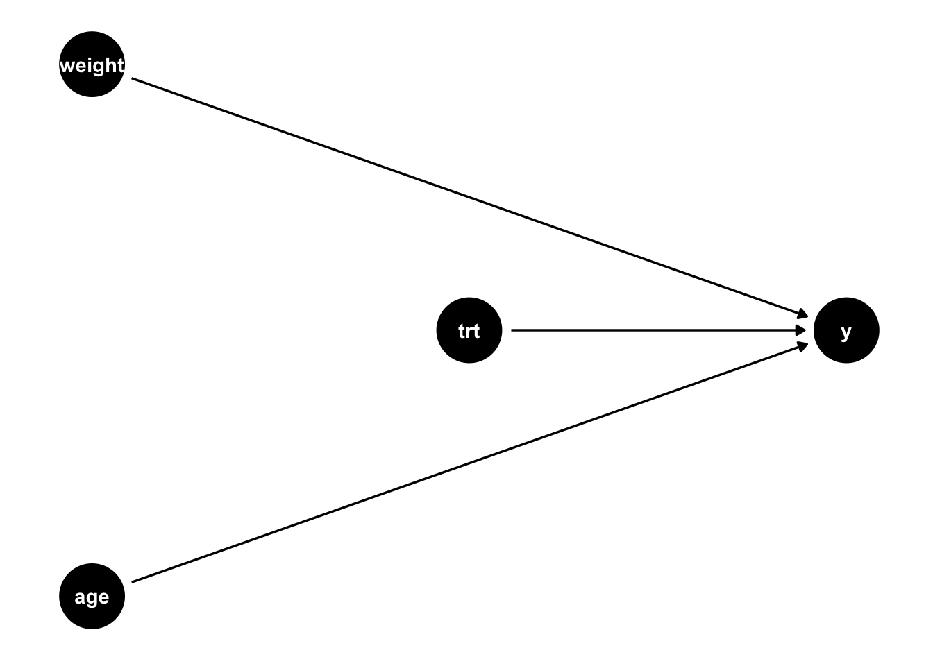
)We can draw a causal diagram of the relationship described in the code above (Figure 4.2). Chapter 5 contains more information on these causal diagrams, but briefly, the arrows denote causal relationships, so since we have established that the treatment causes an increase in the outcome (an average treatment effect of 1), we see an arrow from trt to y in this diagram.
Let’s examine three models: (1) an unadjusted model (Table 4.3 (a)), (2) a linear model that adjusts for the baseline covariates (Table 4.4), and (3) a propensity score weighted model (Table 4.3 (c)).
Code
library(gtsummary)
lm(y ~ treatment, d) |>
  tbl_regression() |>
  modify_column_unhide(column = std.error) |>
modify_caption("Unadjusted regression")| Characteristic | Beta | SE1 | 95% CI1 | p-value |
|---|---|---|---|---|
| treatment | 0.93 | 0.803 | -0.66, 2.5 | 0.2 |
| 1 SE = Standard Error, CI = Confidence Interval | ||||
Code
lm(y ~ treatment + age + weight, d) |>
  tbl_regression() |>
  modify_column_unhide(column = std.error) |>
modify_caption("Adjusted regression")| Characteristic | Beta | SE1 | 95% CI1 | p-value |
|---|---|---|---|---|
| treatment | 1.0 | 0.204 | 0.59, 1.4 | |
| age | 0.20 | 0.005 | 0.19, 0.22 | |
| weight | 0.34 | 0.106 | 0.13, 0.55 | 0.002 |
| 1 SE = Standard Error, CI = Confidence Interval | ||||
Code
d |>
  mutate(
    p = glm(treatment ~ weight + age, data = d) |> predict(type = "response"),
    ate = treatment / p + (1 - treatment) / (1 - p)
  ) |>
  as.data.frame() -> d
library(PSW)
df <- as.data.frame(d)
x <- psw(
  df,
  "treatment ~ weight + age",
  weight = "ATE",
  wt = TRUE,
  out.var = "y"
)
tibble(
  Characteristic = "treatment",
  Beta = round(x$est.wt, 1),
  SE = round(x$std.wt, 3),
  `95% CI` = glue::glue("{round(x$est.wt - 1.96 * x$std.wt, 1)}, {round(x$est.wt + 1.96 * x$std.wt, 1)}"),
  `p-value` = "<0.001"
) |>
knitr::kable(caption = "Propensity score weighted regression")| Characteristic | Beta | SE | 95% CI | p-value |
|---|---|---|---|---|
| treatment | 1 | 0.202 | 0.6, 1.4 | <0.001 |
Table 4.3: Three ways to estimate the causal effect.
Looking at the three outputs in Table 4.3, we can first notice that all three are “unbiased” estimates of the causal effect (we know the true average treatment effect is 1, based on our simulation) – the estimated causal effect in each table is in the Beta column. Great, so all methods give us an unbiased estimate. Next, let’s look at the SE (standard error) column along with the 95% CI (confidence interval) column. Notice the unadjusted model has a wider confidence interval (in fact, in this case the confidence interval includes the null, 0) – this means if we were to use this method, even though we were able to estimate an unbiased causal effect, we would often conclude that we fail to reject the null that relationship between the treatment and outcome is 0. In statistical terms, we refer to this as a lack of efficiency. Looking at the adjusted analysis in Table 4.4, we see that the standard error is quite a bit smaller (and likewise the confidence interval is tighter, no longer including the null). Even though our baseline covariates age and weight were not confounders adjusting from them increased the precision of our result (this is a good thing! We want estimates that are both unbiased and precise). Finally, looking at the propensity score weighted estimate we can see that our precision was slightly improved compared to the adjusted result (0.202 compared to 0.204). The magnitude of this improvement will depend on several factors, but it has been shown mathematically that using propensity scores like this to adjust for baseline factors in a randomized trial will always improve precision (Williamson, Forbes, and White 2014). What can we learn from this small demonstration? Even in the perfect scenario, where we can estimate unbiased results without using propensity scores, the methods we will show here can be useful. The utility of these methods only increases when exploring more complex examples, such as situations where the effect is not randomized, the introduction of time-varying confounders, etc.
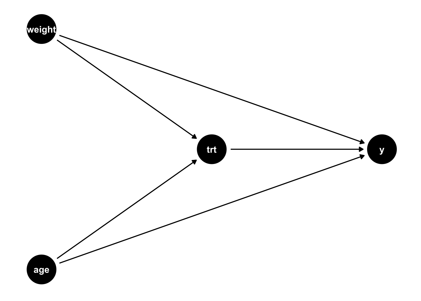
What if we did not have a randomized exposure? There are many cases where randomization to a treatment is not ethical or feasible. Standard methods can still estimate unbiased effects, but more care needs to be given to the previously mentioned assumptions (Table 4.1). For example, we need the exposed an unexposed groups to be exchangeable; this means we must adjust for all confounders with their correct functional form. If everything is simple and linear (and there is no effect heterogeneity, that is everyone’s causal effect is the same regardless of their baseline factors), then a simple regression model that adjusts for the confounders can give you an unbiased result. Let’s look at a simple example such as this. Notice in the simulation below, the main difference compared to the above simulation is that the probability of treatment assignment is no longer 0.5 as it was above, but now dependent on the participants age and weight. For example, maybe doctors tend to prescribe a certain treatment to patients who are older and who weigh more. The true causal effect is still 1, but now we have two confounders, age and weight (Figure 4.3).
set.seed(7)
n <- 100000
d <- tibble(
  age = rnorm(n, 55, 20),
  weight = rnorm(n),
  # generate the treatment from a binomial distribution
  # with the probability of treatment dependent on the age and weight
  treatment = rbinom(n, 1, 1 / (1 + exp(-0.01 * age - weight))),
  ## generate the true average causal effect of the treatment: 1
  y = 1 * treatment + 0.2 * age + 0.2 * weight + rnorm(n)
)
Code
lm(y ~ treatment, d) |>
  tbl_regression() |>
  modify_column_unhide(column = std.error) |>
modify_caption("Unadjusted regression")| Characteristic | Beta | SE1 | 95% CI1 | p-value |
|---|---|---|---|---|
| treatment | 1.8 | 0.027 | 1.8, 1.9 | |
| 1 SE = Standard Error, CI = Confidence Interval | ||||
Code
lm(y ~ treatment + age + weight, d) |>
  tbl_regression() |>
  modify_column_unhide(column = std.error) |>
modify_caption("Adjusted regression")| Characteristic | Beta | SE1 | 95% CI1 | p-value |
|---|---|---|---|---|
| treatment | 0.99 | 0.007 | 0.98, 1.0 | |
| age | 0.20 | 0.000 | 0.20, 0.20 | |
| weight | 0.20 | 0.003 | 0.20, 0.21 | |
| 1 SE = Standard Error, CI = Confidence Interval | ||||
Code
d |>
  mutate(
    p = glm(treatment ~ weight + age, data = d, family = binomial) |> predict(type = "response"),
    ate = treatment / p + (1 - treatment) / (1 - p)
  ) |>
  as.data.frame() -> d
library(PSW)
df <- as.data.frame(d)
x <- psw(
  df,
  "treatment ~ weight + age",
  weight = "ATE",
  wt = TRUE,
  out.var = "y"
)
tibble(
  Characteristic = "treatment",
  Beta = round(x$est.wt, 1),
  SE = round(x$std.wt, 3),
  `95% CI` = glue::glue("{round(x$est.wt - 1.96 * x$std.wt, 1)}, {round(x$est.wt + 1.96 * x$std.wt, 1)}"),
  `p-value` = "<0.001"
) |>
knitr::kable(caption = "Propensity score weighted regression")| Characteristic | Beta | SE | 95% CI | p-value |
|---|---|---|---|---|
| treatment | 1 | 0.014 | 1, 1 | <0.001 |
Table 4.4: Three ways to estimate a causal effect in a non-randomized setting
First, let’s look at Table 4.4 (a). Here, we see that the unadjusted effect is biased (it differs from the true effect, 1, and the true effect is not contained in the reported 95% confidence interval). Now let’s compare Table 4.4 (b) and Table 4.4 (c). Technically, both are estimating unbiased causal effects. The output in the Beta column of Table 4.4 (b) is technically a conditional effect (and often in causal inference we want marginal effects), but because there is no treatment heterogeneity in this simulation, the conditional and marginal effects are equal. Table 4.4 (c), using the propensity score, also estimates an unbiased effect, but it is no longer the most efficient (that was true when the baseline covariates were merely causal for y, now that they are confounders the efficiency gains for using propensity score weighting are not as clear cut). So why would we ever use propensity scores in this case? Sometimes we have a better understanding of the functional form of the propensity score model compared to the outcome model. Alternatively, sometimes the outcome model is difficult to fit (for example, if the outcome is rare).
Marginal versus conditional effects
In causal inference, we are often interested in marginal effects, mathematically, this means that we want to marginalize the effect of interest across the distribution of factors in a particular population that we are trying to estimate a causal effect for. In an adjusted regression model, the coefficients are conditional, in other words, when describing the estimated coefficient, we often say something like “a one-unit change in the exposure results in a coefficient change in the outcome holding all other variables in the model constant. In the case where the outcome is continuous, the effect is linear, and there are no interactions between the exposure effect and other factors about the population, the distinction between an conditional and a marginal effect is largely semantic. If there is an interaction in the model, that is, if the exposure has a different impact on the outcome depending on some other factor, we no longer have a single coefficient to interpret. We would want to estimate a marginal effect, taking into account the distribution of that factor in the population of interest. Why? We are ultimately trying to determine whether we should suggest the exposure to the target population, so we want to know on average whether it will be beneficial. Let’s look at quick example: suppose that you are designing an online shopping site. Currently, the”Purchase” button is grey. Changing the button to red increases revenue by $10 for people who are not colorblind and decreases revenue by $10 for those who are colorblind – the effect is heterogeneous. Whether you change the color of the button will depend on the distribution of colorblind folks that visit your website. For example, if 50% of the visitors are colorblind, your average effect of changing the color would be $0. If instead, 100% are colorblind, the average effect of changing the color would be -$10. Likewise, if 0% are colorblind, the average effect of changing the color to red would be $10. Your decision, therefore, needs to be based on the marginal effect, the effect that takes into account the distribution of colorblind online customers.