n <- 1000000
tibble(
  roll_1 = sample(1:6, n, replace = TRUE),
  roll_2 = sample(1:6, n, replace = TRUE),
) |>
  reframe(roll_1 + roll_2 == 2) |>
  pull() |>
  sum()/n
[1] 0.02787Let’s pause to recap a typical goal of the causal analyses we’ve seen in this book so far: to estimate what would happen if everyone in the study were exposed versus what would happen if no one was exposed. To do this, we’ve used weighting techniques that create confounder-balanced pseudopopulations which, in turn, give rise to unbiased causal effect estimates in marginal outcome models. One alternative approach to weighting is called the parametric G-formula, which is generally executed through the following 4 steps:
Draw the appropriate time ordered DAG (as described in Chapter 5).
For each point in time after baseline, decide on a parametric model that predicts each variable’s value based on previously measured variables in the DAG. These are often linear models for continuous variables or logistic regressions for binary variables.
Starting with a sample from the observed distribution of data at baseline, generate values for all subsequent variables according to the models in step 2 (i.e. conduct a Monte Carlo simulation). Do this with one key modification: for each exposure regime you are interested in comparing (e.g. everyone exposed versus everyone unexposed), assign the exposure variables accordingly (that is, don’t let the simulation assign values for exposure variables).
Compute the causal contrast of interest based on the simulated outcome in each exposure group.
Monte Carlo simulations are computational approaches that generate a sample of outcomes for random processes. One example would be to calculate the probability of rolling “snake eyes” (two ones) on a single roll of two six-sided dice. We could certainly calculate this probability mathematically (\(\frac{1}{6}*\frac{1}{6}=\frac{1}{36}\approx 2.8\)%), though it can be just as quick to write a Monte Carlo simulation of the process (1,000,000 rolls shown below).
n <- 1000000
tibble(
roll_1 = sample(1:6, n, replace = TRUE),
roll_2 = sample(1:6, n, replace = TRUE),
) |>
reframe(roll_1 + roll_2 == 2) |>
pull() |>
sum()/n[1] 0.02787Monte Carlo simulations are extremely useful for estimating outcomes of complex processes for which closed mathematical solutions are not easy to determine. Indeed, that’s why Monte Carlo simulations are so useful for the real-world causal mechanisms described in this book!
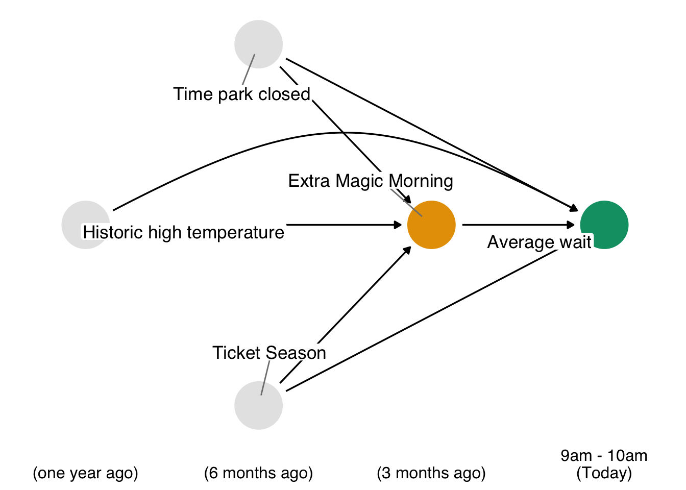
Recall in Chapter 12 that we estimated the impact of extra magic morning hours on the average posted wait time for the Seven Dwarfs ride between 9 and 10am. To do so, we fit a propensity score model for the exposure (park_extra_magic_morning) with the confounders park_ticket_season, park_close, and park_temperature_high. In turn, these propensity scores were converted to regression weights for the outcome model, which concluded that the expected impact of having extra magic hours on the average posted wait time between 9 and 10am is 6.2 minutes.
We will now reproduce this analysis, instead adopting the g-formula approach. Proceeding through the 4 steps outlined above, we begin by revisiting the time ordered DAG relevant to this question.
The second step is to specify a parametric model for each non-baseline variable that is based upon previously measured variables in the DAG. This particular example is simple, since we only have two variables that are affected by previous features (park_extra_magic_morning and wait_minutes_posted_avg). Let’s suppose that adequate models for these two variables are the simple logistic and linear models that follow. Of note, we’re not yet going to use the model for the exposure (park_extra_magic_morning), but we’re including the step here because it will be an important part of patterns you will see in the next section (Section 15.4).
# Load packages and data
library(broom)
library(touringplans)

seven_dwarfs_9 <- seven_dwarfs_train_2018 |>
  filter(wait_hour == 9)

# A logistic regression for park_extra_magic_morning
fit_extra_magic <- glm(
  park_extra_magic_morning ~
    park_ticket_season + park_close + park_temperature_high,
  data = seven_dwarfs_9,
  family = "binomial"
)

# A linear model for wait_minutes_posted_avg
fit_wait_minutes <- lm(
  wait_minutes_posted_avg ~
    park_extra_magic_morning + park_ticket_season + park_close +
    park_temperature_high,
  data = seven_dwarfs_9
)
Next, we need to draw a large sample from the distribution of baseline characteristics. Deciding how large this sample should be is typically based on computational availability; larger sample sizes can minimize the risk of precision loss via simulation error (Keil et al. 2014). In the present case, we’ll use sampling with replacement to generate a data frame of size 10,000.
# It's important to set seeds for reproducibility in Monte Carlo runs
set.seed(8675309)

df_sim_baseline <- seven_dwarfs_9 |>
  select(park_ticket_season, park_close, park_temperature_high) |>
  sample_n(10000, replace = TRUE)
With this population in hand, we can now simulate what would happen at each subsequent time point according to the parametric models we just defined. Remember that, in step 3, an important caveat is that for the variable upon which we wish to intervene (in this case, park_extra_magic_morning) we don’t need to let the model determine the values; rather, we set them. Specifically, we’ll set the first 5000 to park_extra_magic_morning = 1 and the second 5000 to park_extra_magic_morning = 0. Other simulations (in this case, the only remaining variable, wait_minutes_posted_avg) proceed as expected.
# Set the exposure groups for the causal contrast we wish to estimate
df_sim_time_1 <- df_sim_baseline |>
  mutate(park_extra_magic_morning = c(rep(1, 5000), rep(0, 5000)))

# Simulate the outcome according to the parametric model in step 2
df_outcome <- fit_wait_minutes |>
  augment(newdata = df_sim_time_1) |>
  rename(wait_minutes_posted_avg = .fitted)
All that is left to do is compute the causal contrast we wish to estimate. Here, that contrast is the difference between expected wait minutes on extra magic mornings versus mornings without the extra magic program.
df_outcome |>
  group_by(park_extra_magic_morning) |>
  summarize(wait_minutes = mean(wait_minutes_posted_avg))
# A tibble: 2 × 2
park_extra_magic_morning wait_minutes
<dbl> <dbl>
1 0 68.1
2 1 74.3We see that the difference, \(74.3-68.1=6.2\) is the same as our estimate of 6.2 when we used IP weighting.
As previously mentioned, a key strength of the g-formula is its capacity to handle continuous exposures, a situation in which IP weighting can give rise to unstable estimates. Here, we briefly repeat the example from Chapter 13 to show how this is done. To extend the pattern, we will wrap this execution of the technique in a bootstrap to show how confidence intervals are computed.
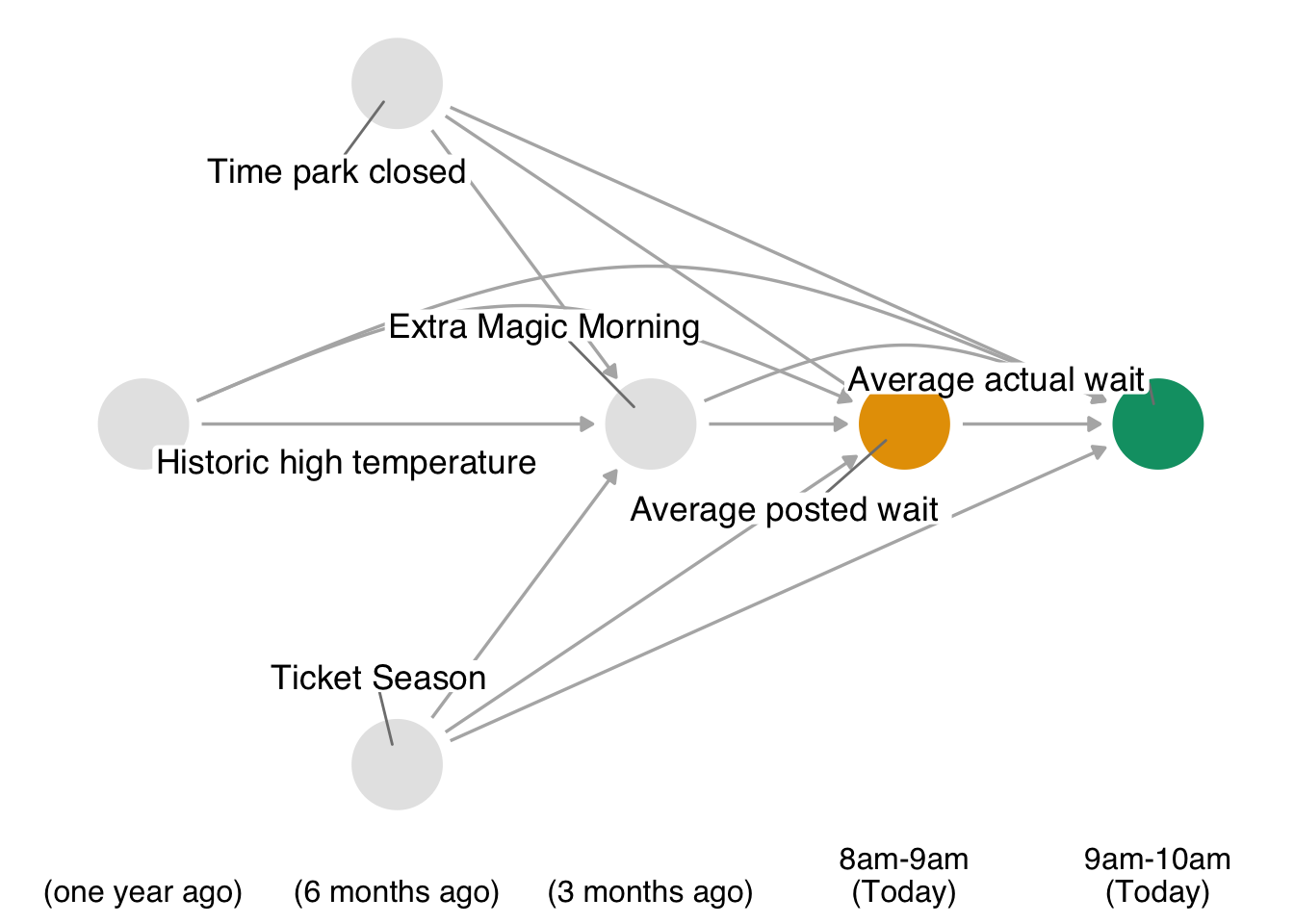
Recall, our causal question of interest is “Do posted wait times for the Seven Dwarfs Mine Train at 8 am affect actual wait times at 9 am?” The time-ordered DAG for this question (step 1) is:
For step 2, we need to specify parametric models for the non-baseline variables in our DAG (i.e. any variables which have arrows into them). In this case, we need such models for park_extra_magic_morning, wait_minutes_posted_avg, and wait_minutes_actual_avg; we’ll assume that the below logistic and linear models are appropriate. One extension to our previous implementation is that we’re going to embed the each step of the process into a function, since this will allow us to bootstrap the entire pipeline and obtain confidence intervals.
library(splines)

fit_models <- function(.data) {

  # A logistic regression for park_extra_magic_morning
  fit_extra_magic <- glm(
    park_extra_magic_morning ~
      park_ticket_season + park_close + park_temperature_high,
    data = .data,
    family = "binomial"
  )

  # A linear model for wait_minutes_posted_avg
  fit_wait_minutes_posted <- lm(
    wait_minutes_posted_avg ~
      park_extra_magic_morning + park_ticket_season + park_close +
      park_temperature_high,
    data = .data
  )

  # A linear model for wait_minutes_actual_avg
  # Let's go ahead an add a spline for further flexibility.
  # Be aware this is an area where you can add many options here
  # (interactions, etc) but you may get warnings and/or models which
  # fail to converge if you don't have enough data.
  fit_wait_minutes_actual <- lm(
    wait_minutes_actual_avg ~
      ns(wait_minutes_posted_avg, df = 3) +
      park_extra_magic_morning +
      park_ticket_season + park_close +
      park_temperature_high,
    data = .data
  )

  # return a list that we can pipe into our simulation step (up next)
  return(
    list(
      .data = .data,
      fit_extra_magic = fit_extra_magic,
      fit_wait_minutes_posted = fit_wait_minutes_posted,
      fit_wait_minutes_actual = fit_wait_minutes_actual
    )
  )

}
Next, we write a function which will complete step 3: from a random sample from the distribution of baseline variables, generate values for all subsequent variables (except the intervention variable) according to the models we defined.
# The arguments to simulate_process are as follows:
# fit_obj is a list which is returned from our fit_models function
# contrast gives exposure (default 60) and control group (default 30) settings
# n_sample is the size of the baseline resample of .data
simulate_process <- function(
    fit_obj,
    contrast = c(60, 30),
    n_sample = 10000
) {

  # Draw a random sample of baseline variables
  df_baseline <- fit_obj |>
    pluck(".data") |>
    select(park_ticket_season, park_close, park_temperature_high) |>
    sample_n(n_sample, replace = TRUE)

  # Simulate park_extra_magic_morning
  df_sim_time_1 <- fit_obj |>
    pluck("fit_extra_magic") |>
    augment(newdata = df_baseline, type.predict = "response") |>
    # .fitted is the probability that park_extra_magic_morning is 1,
    # so let's use that to generate a 0/1 outcome
    mutate(
      park_extra_magic_morning = rbinom(n(), 1, .fitted)
    )

  # Assign wait_minutes_posted_avg, since it's the intervention
  df_sim_time_2 <- df_sim_time_1 |>
    mutate(
      wait_minutes_posted_avg =
        c(rep(contrast[1], n_sample/2), rep(contrast[2], n_sample/2))
    )

  # Simulate the outcome
  df_outcome <- fit_obj |>
    pluck("fit_wait_minutes_actual") |>
    augment(newdata = df_sim_time_2) |>
    rename(wait_minutes_actual_avg = .fitted)

  # return a list that we can pipe into the contrast estimation step (up next)
  return(
    list(
      df_outcome = df_outcome,
      contrast = contrast
    )
  )
}
Finally, in step 4, we compute the summary statistics and causal contrast of interest using our simulated data.
# sim_obj is a list created by our simulate_process() function
compute_stats <- function(sim_obj) {

  exposure_val <- sim_obj |>
    pluck("contrast", 1)

  control_val <- sim_obj |>
    pluck("contrast", 2)

  sim_obj |>
    pluck("df_outcome") |>
    group_by(wait_minutes_posted_avg) |>
    summarize(avg_wait_actual = mean(wait_minutes_actual_avg)) |>
    pivot_wider(
      names_from = wait_minutes_posted_avg,
      values_from = avg_wait_actual,
      names_prefix = "x_"
    ) |>
    summarize(
      x_60, x_30, x_60 - x_30
    )

}
Now, let’s put it all together to get a single point estimate. Once we’ve seen that in action, we’ll bootstrap for a confidence interval.
# Wrangle the data to reflect the causal question we are asking
eight <- seven_dwarfs_train_2018 |>
  filter(wait_hour == 8) |>
  select(-wait_minutes_actual_avg)

nine <- seven_dwarfs_train_2018 |>
  filter(wait_hour == 9) |>
  select(park_date, wait_minutes_actual_avg)

wait_times <- eight |>
  left_join(nine, by = "park_date") |>
  drop_na(wait_minutes_actual_avg)

# get a single point estimate to make sure things work as we planned
wait_times |>
  fit_models() |>
  simulate_process() |>
  compute_stats() |>
  # rsample wants results labelled this way
  pivot_longer(
    names_to = "term",
    values_to = "estimate",
    cols = everything()
  )
# A tibble: 3 × 2
term estimate
<chr> <dbl>
1 x_60 29.9
2 x_30 40.6
3 x_60 - x_30 -10.7# compute bootstrap confidence intervals
library(rsample)
boots <- bootstraps(wait_times, times = 1000, apparent = TRUE) |>
mutate(
models = map(
splits,
\(.x) analysis(.x) |>
fit_models() |>
simulate_process() |>
compute_stats() |>
pivot_longer(
names_to = "term",
values_to = "estimate",
cols = everything()
)
)
)Warning: There was 1 warning in `mutate()`.
ℹ In argument: `models = map(...)`.
Caused by warning:
! glm.fit: fitted probabilities numerically 0 or 1 occurredresults <- int_pctl(boots, models)
results# A tibble: 3 × 6
term .lower .estimate .upper .alpha .method
<chr> <dbl> <dbl> <dbl> <dbl> <chr>
1 x_30 33.1 40.6 48.8 0.05 percentile
2 x_60 14.0 30.5 47.6 0.05 percentile
3 x_60 - x_30 -30.8 -10.0 11.7 0.05 percentileIn summary, our results are intepreted as follows: setting the posted wait time at 8am to 60 minutes results in an actual wait time at 9am of 31, while setting the posted wait time to 30 minutes gives a longer wait time of 41. Put another way, increasing the posted wait time at 8am from 30 minutes to 60 minutes results in a 10 minute shorter wait time at 9am.
Note that one of our models threw a warning regarding perfect discrimination (fitted probabilities numerically 0 or 1 occurred); this can happen when we don’t have a large sample size and one of our models is overspecified due to complexity. In this exercise, the flexibility added by the spline in the regression for wait_minutes_actual_avg is what caused the issue. One remedy when this happens is to simplify the offending model (i.e. if you modify the wait_minutes_actual_avg to include a simple linear term for wait_minutes_posted_avg), the warning is resolved. We’ve left the warning here to highlight a common challenge that needs resolution when working with the parametric g-formula on small- to mid-sized data sets.