library(broom)
library(touringplans)
library(MatchIt)

seven_dwarfs_9 <- seven_dwarfs_train_2018 |>
  filter(wait_hour == 9)

m <- matchit(
  park_extra_magic_morning ~ park_ticket_season + park_close + park_temperature_high,
  data = seven_dwarfs_9
)
matched_data <- get_matches(m)12 Fitting the outcome model
12.1 Using matched data sets
When fitting an outcome model on matched data sets, we can simply subset the original data to only those who were matched and then fit a model on these data as we would otherwise. For example, re-performing the matching as we did in Chapter 9, we can extract the matched observations in a dataset called matched_data as follows.
We can then fit the outcome model on this data. For this analysis, we are interested in the impact of extra magic morning hours on the average posted wait time between 9 and 10am. The linear model below will estimate this in the matched cohort.
lm(wait_minutes_posted_avg ~ park_extra_magic_morning, data = matched_data) |>
  tidy(conf.int = TRUE)
# A tibble: 2 × 7
term estimate std.error statistic p.value conf.low
<chr> <dbl> <dbl> <dbl> <dbl> <dbl>
1 (Inte… 67.0 2.37 28.3 1.94e-54 62.3
2 park_… 7.87 3.35 2.35 2.04e- 2 1.24
# ℹ 1 more variable: conf.high <dbl>Recall that by default MatchIt estimates an average treatment effect among the treated. This means among days that have extra magic hours, the expected impact of having extra magic hours on the average posted wait time between 9 and 10am is 7.9 minutes (95% CI: 1.2-14.5).
12.2 Using weights in outcome models
Now let’s use propensity score weights to estimate this same estimand. We will use the ATT weights so the analysis matches that for matching above.
library(propensity)

seven_dwarfs_9_with_ps <-
  glm(
    park_extra_magic_morning ~ park_ticket_season + park_close + park_temperature_high,
    data = seven_dwarfs_9,
    family = binomial()
  ) |>
  augment(type.predict = "response", data = seven_dwarfs_9)
seven_dwarfs_9_with_wt <- seven_dwarfs_9_with_ps |>
  mutate(w_att = wt_att(.fitted, park_extra_magic_morning))
We can fit a weighted outcome model by using the weights argument.
lm(
  wait_minutes_posted_avg ~ park_extra_magic_morning,
  data = seven_dwarfs_9_with_wt,
  weights = w_att
) |>
  tidy()
# A tibble: 2 × 5
term estimate std.error statistic p.value
<chr> <dbl> <dbl> <dbl> <dbl>
1 (Intercept) 68.7 1.45 47.3 1.69e-154
2 park_extra_ma… 6.23 2.05 3.03 2.62e- 3Using weighting, we estimate that among days that have extra magic hours, the expected impact of having extra magic hours on the average posted wait time between 9 and 10am is 6.2 minutes. While this approach will get us the desired estimate for the point estimate, the default output using the lm function for the uncertainty (the standard errors and confidence intervals) are not correct.
12.3 Estimating uncertainty
There are three ways to estimate the uncertainty:
- A bootstrap
- A sandwich estimator that only takes into account the outcome model
- A sandwich estimator that takes into account the propensity score model
The first option can be computationally intensive, but should get you the correct estimates. The second option is computationally the easiest, but tends to overestimate the variability. There are not many current solutions in R (aside from coding it up yourself) for the third; however, the {PSW} package will do this.
12.3.1 The bootstrap
- Create a function to run your analysis once on a sample of your data
fit_ipw <- function(split, ...) {
  .df <- analysis(split)

  # fit propensity score model
  propensity_model <- glm(
    park_extra_magic_morning ~ park_ticket_season + park_close + park_temperature_high,
    data = seven_dwarfs_9,
    family = binomial()
  )

  # calculate inverse probability weights
  .df <- propensity_model |>
    augment(type.predict = "response", data = .df) |>
    mutate(wts = wt_att(
      .fitted,
      park_extra_magic_morning,
      exposure_type = "binary"
    ))

  # fit correctly bootstrapped ipw model
  lm(
    wait_minutes_posted_avg ~ park_extra_magic_morning,
    data = .df,
    weights = wts
  ) |>
    tidy()
}- Use {rsample} to bootstrap our causal effect
library(rsample)

# fit ipw model to bootstrapped samples
bootstrapped_seven_dwarfs <- bootstraps(
  seven_dwarfs_9,
  times = 1000,
  apparent = TRUE
)

ipw_results <- bootstrapped_seven_dwarfs |>
  mutate(boot_fits = map(splits, fit_ipw))

ipw_results
# Bootstrap sampling with apparent sample
# A tibble: 1,001 × 3
splits id boot_fits
<list> <chr> <list>
1 <split [354/128]> Bootstrap0001 <tibble [2 × 5]>
2 <split [354/132]> Bootstrap0002 <tibble [2 × 5]>
3 <split [354/132]> Bootstrap0003 <tibble [2 × 5]>
4 <split [354/135]> Bootstrap0004 <tibble [2 × 5]>
5 <split [354/125]> Bootstrap0005 <tibble [2 × 5]>
6 <split [354/132]> Bootstrap0006 <tibble [2 × 5]>
7 <split [354/126]> Bootstrap0007 <tibble [2 × 5]>
8 <split [354/121]> Bootstrap0008 <tibble [2 × 5]>
9 <split [354/136]> Bootstrap0009 <tibble [2 × 5]>
10 <split [354/128]> Bootstrap0010 <tibble [2 × 5]>
# ℹ 991 more rowsLet’s look at the results.
ipw_results |>
  mutate(
    estimate = map_dbl(
      boot_fits,
      \(.fit) .fit |>
        filter(term == "park_extra_magic_morning") |>
        pull(estimate)
    )
  ) |>
  ggplot(aes(estimate)) +
  geom_histogram(bins = 30, fill = "#D55E00FF", color = "white", alpha = 0.8) +
  theme_minimal()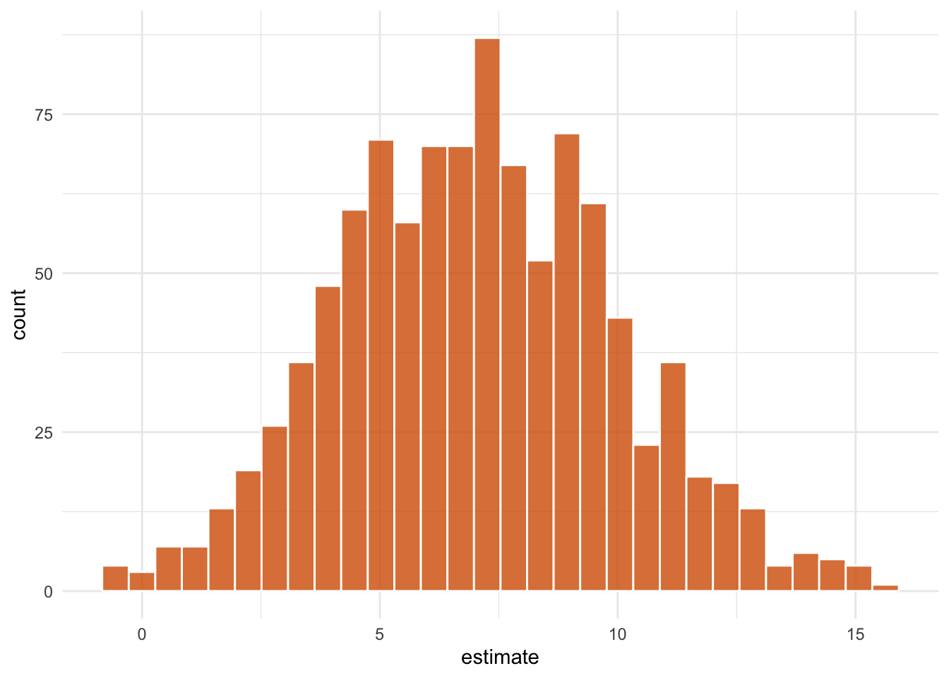
- Pull out the causal effect
# get t-based CIs
boot_estimate <- int_t(ipw_results, boot_fits) |>
  filter(term == "park_extra_magic_morning")
boot_estimate
# A tibble: 1 × 6
term .lower .estimate .upper .alpha .method
<chr> <dbl> <dbl> <dbl> <dbl> <chr>
1 park_extra_ma… -0.336 7.05 11.1 0.05 studen…We estimate that among days that have extra magic hours, the expected impact of having extra magic hours on the average posted wait time between 9 and 10am is 7.1 minutes, 95% CI (-0.3, 11.1).
12.3.2 The outcome model sandwich
There are two ways to get the sandwich estimator. The first is to use the same weighted outcome model as above along with the sandwich package. Using the sandwich function, we can get the robust estimate for the variance for the parameter of interest, as shown below.
library(sandwich)
weighted_mod <- lm(
  wait_minutes_posted_avg ~ park_extra_magic_morning,
  data = seven_dwarfs_9_with_wt,
  weights = w_att
)

sandwich(weighted_mod)
(Intercept)
(Intercept) 1.488
park_extra_magic_morning -1.488
park_extra_magic_morning
(Intercept) -1.488
park_extra_magic_morning 8.727Here, our robust variance estimate is 8.727. We can then use this to construct a robust confidence interval.
robust_var <- sandwich(weighted_mod)[2, 2]
point_est <- coef(weighted_mod)[2]
lb <- point_est - 1.96 * sqrt(robust_var)
ub <- point_est + 1.96 * sqrt(robust_var)
lb
park_extra_magic_morning
0.4383 ubpark_extra_magic_morning
12.02 We estimate that among days that have extra magic hours, the expected impact of having extra magic hours on the average posted wait time between 9 and 10am is 6.2 minutes, 95% CI (0.4, 12).
Alternatively, we could fit the model using the survey package. To do this, we need to create a design object, like we did when fitting weighted tables.
Then we can use svyglm to fit the outcome model.
# A tibble: 2 × 7
  term  estimate std.error statistic   p.value conf.low
  <chr>    <dbl>     <dbl>     <dbl>     <dbl>    <dbl>
1 (Int…    68.7       1.22     56.2  6.14e-178   66.3
2 park…     6.23      2.96      2.11 3.60e-  2    0.410
# ℹ 1 more variable: conf.high <dbl>
12.3.3 Sandwich estimator that takes into account the propensity score model
The correct sandwich estimator will also take into account the propensity score model. The {PSW} will allow us to do this. This package has some quirks, for example it doesn’t work well with categorical variables, so we need to create dummy variables for park_ticket_season to pass into the model. Actually, the code below isn’t working because it seems there is a bug in the package. Stay tuned!
library(PSW)

seven_dwarfs_9 <- seven_dwarfs_9 |>
  mutate(
    park_ticket_season_regular = ifelse(park_ticket_season == "regular", 1, 0),
    park_ticket_season_value = ifelse(park_ticket_season == "value", 1, 0)
  )
psw(
  data = seven_dwarfs_9,
  form.ps = "park_extra_magic_morning ~ park_ticket_season_regular + park_ticket_season_value + park_close + park_temperature_high",
  weight = "ATT",
  wt = TRUE,
  out.var = "wait_minutes_posted_avg"
)