13 Continuous exposures
13.1 Calculating propensity scores for continuous exposures
Propensity scores generalize to many other types of exposures, including continuous exposures. At its heart, the workflow is the same: we fit a model where the exposure is the outcome and then use that model to weight a second outcome model. For continuous exposures, linear regression is the simplest way to create propensities. Instead of probabilities, we use the cumulative density function. Then, we use this density to weight the outcome model.
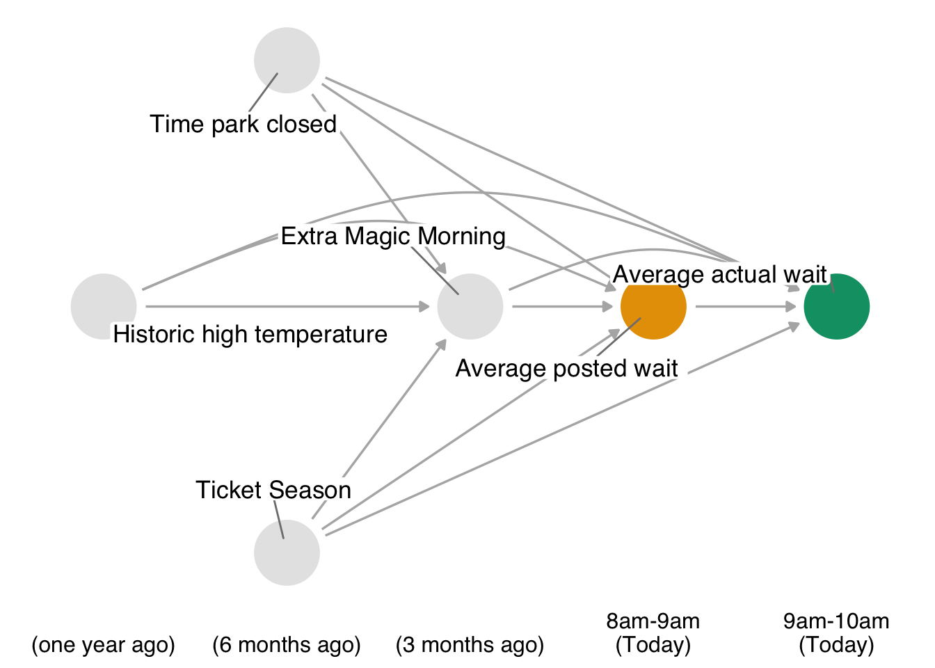
Let’s take a look at an example. In the touringplans data set, we have information about the posted waiting times for rides. We also have a limited amount of data on the observed actual times. The question we will consider is this: Do posted wait times for the Seven Dwarfs Mine Train at 8 am affect actual wait times at 9 am? Here’s our DAG:
In Figure 13.1, we’re assuming that our primary confounders are when the park closes, historic high temperatures, whether or not the ride has extra magic morning hours, and the ticket season. This is the only minimal adjustment set in the DAG, as well. The confounders precede the exposure and outcome, and (by definition) the exposure precedes the outcome. The average posted wait time is, in theory, a manipulable exposure because the park could post a time different from what they expect. The adjustment set
The model is similar to the binary exposure case, but we need to use linear regression, as the posted time is a continuous variable. Since we’re not using probabilities, we’ll calculate denominators for our weights from a normal density. We then calculate the denominator using the dnorm() function, which calculates the normal density for the exposure, using .fitted as the mean and mean(.sigma) as the SD.
13.2 Diagnostics and stabilization
Continuous exposure weights, however, are very sensitive to modeling choices. One problem, in particular, is the existence of extreme weights, an issue that can also affect other types of exposures. When some observations have extreme weights, the propensities are destabilized, which results in wider confidence intervals. We can stabilize them using the marginal distribution of the exposure. A common way to calculate the marginal distribution for propensity scores is to use a regression model with no predictors.
Extreme weights destabilize estimates, resulting in wider confidence intervals. Extreme weights can be an issue for any time of weight (including those for binary and other types of exposures) that is not bounded. Bounded weights like the ATO (which are bounded to 0 and 1) do not have this problem, however—one of their many benefits.
# for continuous exposures
lm(
  exposure ~ 1,
  data = df
) |>
  augment(data = df) |>
  transmute(
    numerator = dnorm(exposure, .fitted, mean(.sigma, na.rm = TRUE))
  )

# for binary exposures
glm(
  exposure ~ 1,
  data = df,
  family = binomial()
) |>
  augment(type.predict = "response", data = df) |>
  select(numerator = .fitted)
Then, rather than inverting them, we calculate the weights as numerator / denominator. Let’s try it out on our posted wait times example. First, let’s wrangle our data to address our question: do posted wait times at 8 affect actual weight times at 9? We’ll join the baseline data (all covariates and posted wait time at 8) with the outcome (average actual time). We also have a lot of missingness for wait_minutes_actual_avg, so we’ll drop unobserved values for now.
library(tidyverse)
library(touringplans)
eight <- seven_dwarfs_train_2018 |>
  filter(wait_hour == 8) |>
  select(-wait_minutes_actual_avg)

nine <- seven_dwarfs_train_2018 |>
  filter(wait_hour == 9) |>
  select(park_date, wait_minutes_actual_avg)

wait_times <- eight |>
  left_join(nine, by = "park_date") |>
  drop_na(wait_minutes_actual_avg)
First, let’s calculate our denominator model. We’ll fit a model using lm() for wait_minutes_posted_avg with our covariates, then use the fitted predictions of wait_minutes_posted_avg (.fitted) to calculate the density using dnorm().
library(broom)
denominator_model <- lm(
  wait_minutes_posted_avg ~
    park_close + park_extra_magic_morning + park_temperature_high + park_ticket_season,
  data = wait_times
)

denominators <- denominator_model |>
  augment(data = wait_times) |>
  mutate(
    denominator = dnorm(
      wait_minutes_posted_avg,
      .fitted,
      mean(.sigma, na.rm = TRUE)
    )
  ) |>
  select(park_date, denominator, .fitted)
When we only use the inverted values of denominator, we end up with several extreme weights:
denominators |>
  mutate(wts = 1 / denominator) |>
  ggplot(aes(wts)) +
  geom_histogram(fill = "#E69F00", color = "white", bins = 50) +
  scale_x_log10(name = "weights")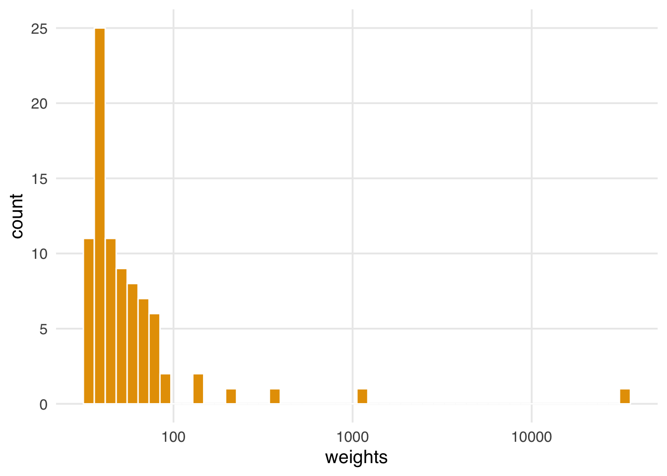
In Figure 13.2, we see several weights over 100 and one over 10,000; these extreme weights will put undue stress on specific points, complicating the results we will estimate.
Let’s now fit the marginal density to use for stabilized weights:
We also need to join the fitted values back to our original data set by date, then calculate the stabilized weights (swts) using numerator / denominator.
The stabilized weights are much less extreme. Stabilized weights should have a mean close to 1 (in this example, it is round(mean(wait_times_wts$swts), digits = 2)); when that is the case, then the pseudo-population (that is, the equivalent number of observations after weighting) is equal to the original sample size. If the mean is far from 1, we may have issues with model misspecification or positivity violations (Hernán and Robins 2021).
ggplot(wait_times_wts, aes(swts)) +
  geom_histogram(fill = "#E69F00", color = "white", bins = 50) +
  scale_x_log10(name = "weights")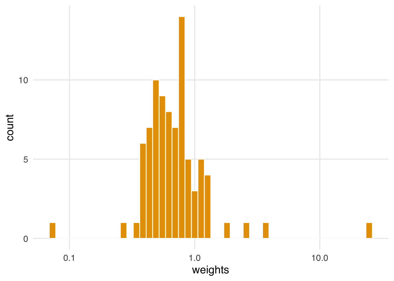
When we compare the exposure—average posted wait times—to the standardized weights, we still have one exceptionally high weight. Is this a problem, or is this a valid data point?
ggplot(wait_times_wts, aes(wait_minutes_posted_avg, swts)) +
  geom_point(size = 3, color = "grey80", alpha = 0.7) +
  geom_point(
    data = function(x) filter(x, swts > 10),
    color = "firebrick",
    size = 3
  ) +
  geom_text(
    data = function(x) filter(x, swts > 10),
    aes(label = park_date),
    size = 5,
    hjust = 0,
    nudge_x = -15.5,
    color = "firebrick"
  ) +
  scale_y_log10() +
  labs(x = "Average Posted Wait", y = "Stabilized Weights")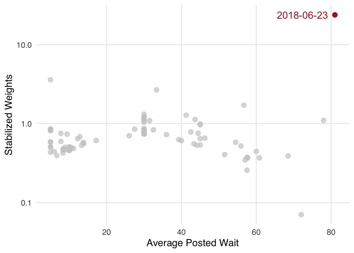
wait_minutes_posted_avg farther from the mean appear to be downweighted, with a few exceptions. The most unusual weight is for June 23, 2018.wait_times_wts |>
filter(swts > 10) |>
select(
park_date,
wait_minutes_posted_avg,
.fitted,
park_close,
park_extra_magic_morning,
park_temperature_high,
park_ticket_season
) |>
knitr::kable()| park_date | wait_minutes_posted_avg | .fitted | park_close | park_extra_magic_morning | park_temperature_high | park_ticket_season |
|---|---|---|---|---|---|---|
| 2018-06-23 | 81 | 28.1 | 24:00:00 | 0 | 91.36 | regular |
Our model predicted a much lower posted wait time than observed, so this date was upweighted. We don’t know why the posted time was so high (the actual time was much lower), but we did find an artist rendering from that date of Pluto digging for Seven Dwarfs Mine Train treasure.