library(quartets)

anscombe_quartet |>
  ggplot(aes(x, y)) +
  geom_point() +
  geom_smooth(method = "lm", se = FALSE) +
  facet_wrap(~ dataset)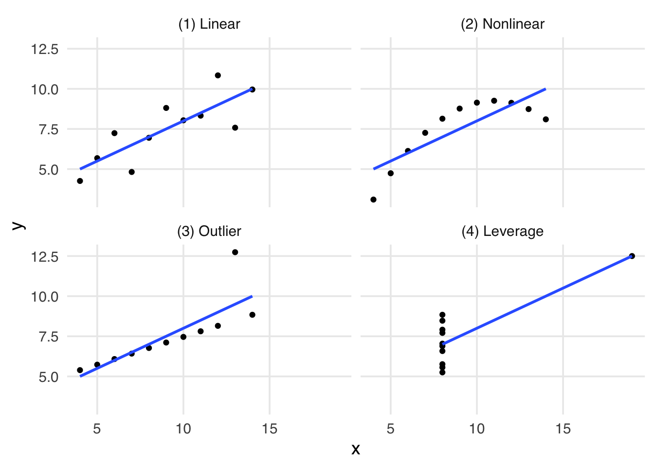
We now have the tools to look at something we’ve alluded to thus far in the book: causal inference is not (just) a statistical problem. Of course, we use statistics to answer causal questions. It’s necessary to answer most questions, even if the statistics are basic (as they often are in randomized designs). However, statistics alone do not allow us to address all of the assumptions of causal inference.
In 1973, Francis Anscombe introduced a set of four datasets called Anscombe’s Quartet. These data illustrated an important lesson: summary statistics alone cannot help you understand data; you must also visualize your data. In the plots in Figure 6.1, each data set has remarkably similar summary statistics, including means and correlations that are nearly identical.
library(quartets)
anscombe_quartet |>
ggplot(aes(x, y)) +
geom_point() +
geom_smooth(method = "lm", se = FALSE) +
facet_wrap(~ dataset)
The Datasaurus Dozen is a modern take on Anscombe’s Quartet. The mean, standard deviation, and correlation are nearly identical in each dataset, but the visualizations are very different.
library(datasauRus)

# roughly the same correlation in each dataset
datasaurus_dozen |>
  group_by(dataset) |>
  summarize(cor = round(cor(x, y), 2))
# A tibble: 13 × 2
dataset cor
<chr> <dbl>
1 away -0.06
2 bullseye -0.07
3 circle -0.07
4 dino -0.06
5 dots -0.06
6 h_lines -0.06
7 high_lines -0.07
8 slant_down -0.07
9 slant_up -0.07
10 star -0.06
11 v_lines -0.07
12 wide_lines -0.07
13 x_shape -0.07datasaurus_dozen |>
ggplot(aes(x, y)) +
geom_point() +
facet_wrap(~ dataset)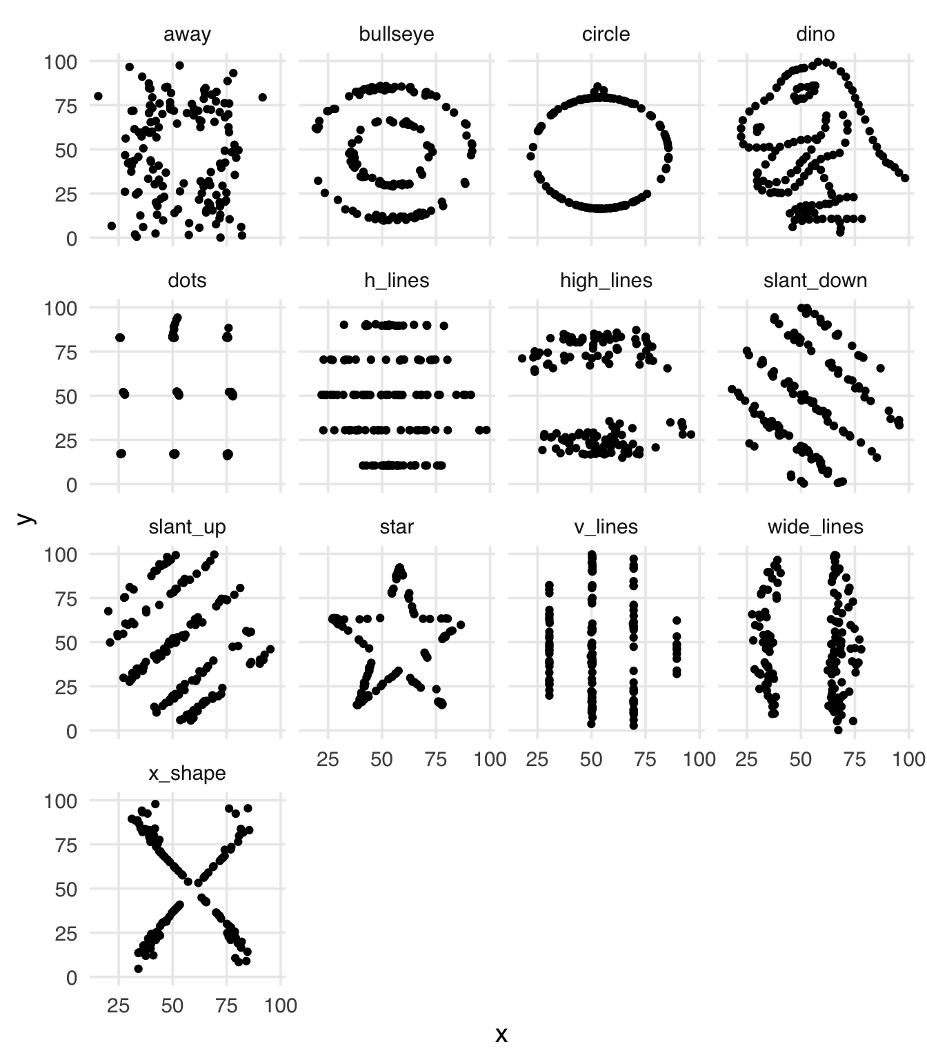
In causal inference, however, even visualization is insufficient to untangle causal effects. As we visualized in DAGs in Chapter 5, background knowledge is required to infer causation from correlation (Robins and Wasserman 1999).
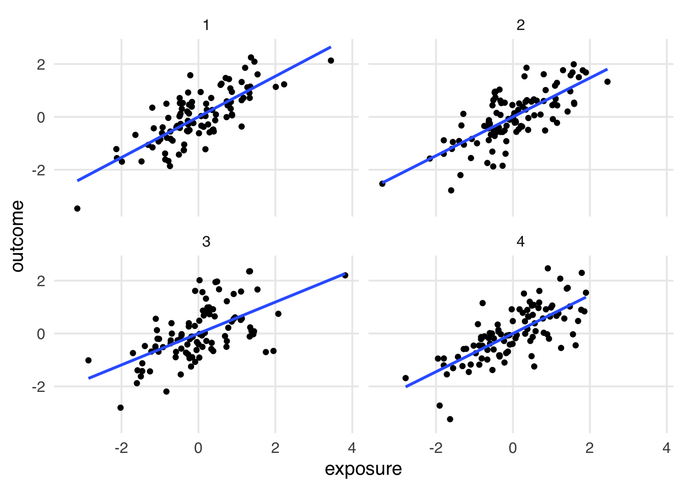
Inspired by Anscombe’s quartet, the causal quartet has many of the same properties of Anscombe’s quartet and the Datasaurus Dozen: the numerical summaries of the variables in the dataset are the same (D’Agostino McGowan, Gerke, and Barrett 2023). Unlike these data, the causal quartet also look the same as each other. The difference is the causal structure that generated each dataset. Figure 6.3 shows four datasets where the observational relationship between exposure and outcome is virtually identical.
causal_quartet |>
  # hide the dataset names
  mutate(dataset = as.integer(factor(dataset))) |>
  group_by(dataset) |>
  mutate(exposure = scale(exposure), outcome = scale(outcome)) |>
  ungroup() |>
  ggplot(aes(exposure, outcome)) +
  geom_point() +
  geom_smooth(method = "lm", se = FALSE) +
facet_wrap(~ dataset)The question for each dataset is whether to adjust for a third variable, covariate. Is covariate a confounder? A mediator? A collider? We can’t use data to figure this problem out. In Table 6.1, it’s not clear which effect is correct. Likewise, the correlation between exposure and covariate is no help: they’re all the same!
| Dataset | Not adjusting for covariate
|
Adjusting for covariate
|
Correlation of exposure and covariate
|
|---|---|---|---|
| 1 | 1.00 | 0.55 | 0.70 |
| 2 | 1.00 | 0.50 | 0.70 |
| 3 | 1.00 | 0.00 | 0.70 |
| 4 | 1.00 | 0.88 | 0.70 |
The ten percent rule is a common technique in epidemiology and other fields to determine whether a variable is a confounder. The ten percent rule says that you should include a variable in your model if including it changes the effect estimate by more than ten percent. The problem is, it doesn’t work. Every example in the causal quartet causes a more than ten percent change. As we know, this leads to the wrong answer in some of the datasets. Even the reverse technique, excluding a variable when it’s less than ten percent, can cause trouble because many minor confounding effects can add up to more considerable bias.
| Dataset | Percent change |
|---|---|
| 1 | 44.6% |
| 2 | 49.7% |
| 3 | 99.8% |
| 4 | 12.5% |
While the visual relationship between covariate and exposure is not identical between datasets, all have the same correlation. In Figure 6.4, the standardized relationship between the two is identical.
causal_quartet |>
  # hide the dataset names
  mutate(dataset = as.integer(factor(dataset))) |>
  group_by(dataset) |>
  summarize(cor = round(cor(covariate, exposure), 2))
# A tibble: 4 × 2
dataset cor
<int> <dbl>
1 1 0.7
2 2 0.7
3 3 0.7
4 4 0.7causal_quartet |>
# hide the dataset names
mutate(dataset = as.integer(factor(dataset))) |>
group_by(dataset) |>
mutate(covariate = scale(covariate), exposure = scale(exposure)) |>
ungroup() |>
ggplot(aes(covariate, exposure)) +
geom_point() +
geom_smooth(method = "lm", se = FALSE) +
facet_wrap(~ dataset) 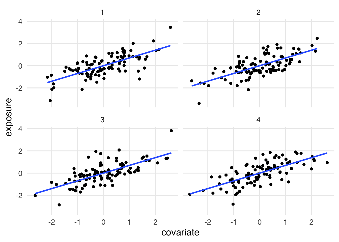
covariate is a confounder, mediator, or collider.Standardizing numeric variables to have a mean of 0 and standard deviation of 1, as implemented in scale(), is a common technique in statistics. It’s useful for a variety of reasons, but we chose to scale the variables here to emphasize the identical correlation between covariate and exposure in each dataset. If we didn’t scale the variables, the correlation would be the same, but the plots would look different because their standard deviation are different. The beta coefficient in an OLS model is calculated with information about the covariance and the standard deviation of the variable, so scaling it makes the coefficient identical to the Pearson’s correlation.
Figure 6.5 shows the unscaled relationship between covariate and exposure. Now, we see some differences: dataset 4 seems to have more variance in covariate, but that’s not actionable information. In fact, it’s a mathematical artifact of the data generating process.
causal_quartet |>
  # hide the dataset names
  mutate(dataset = as.integer(factor(dataset))) |>
  ggplot(aes(covariate, exposure)) +
  geom_point() +
  geom_smooth(method = "lm", se = FALSE) +
  facet_wrap(~ dataset)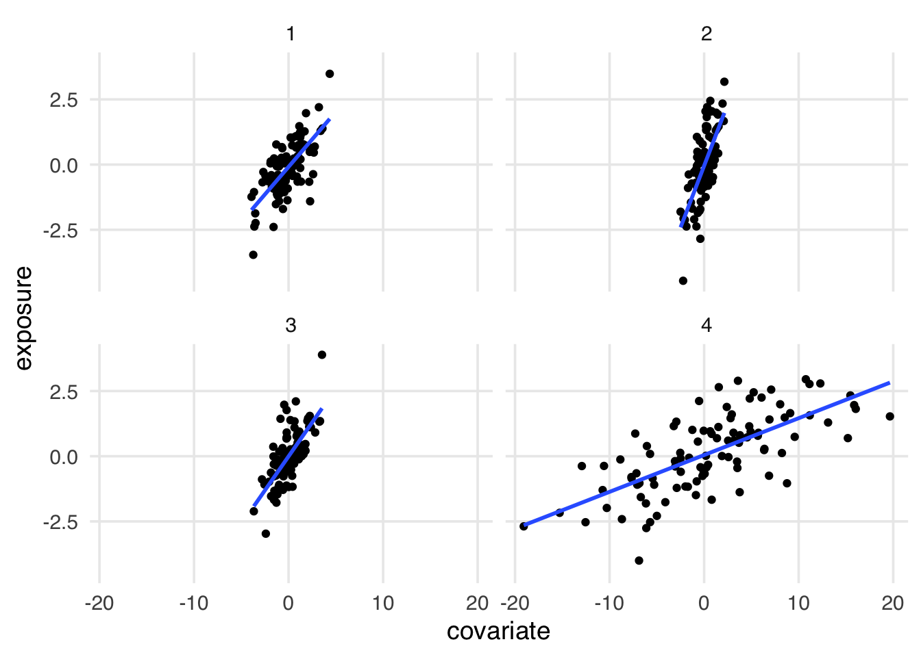
Let’s reveal the labels of the datasets, representing the causal structure of the dataset. Figure 6.6, covariate plays a different role in each dataset. In 1 and 4, it’s a collider (we shouldn’t adjust for it). In 2, it’s a confounder (we should adjust for it). In 3, it’s a mediator (it depends on the research question).
causal_quartet |>
  ggplot(aes(exposure, outcome)) +
  geom_point() +
  geom_smooth(method = "lm", se = FALSE) +
  facet_wrap(~ dataset)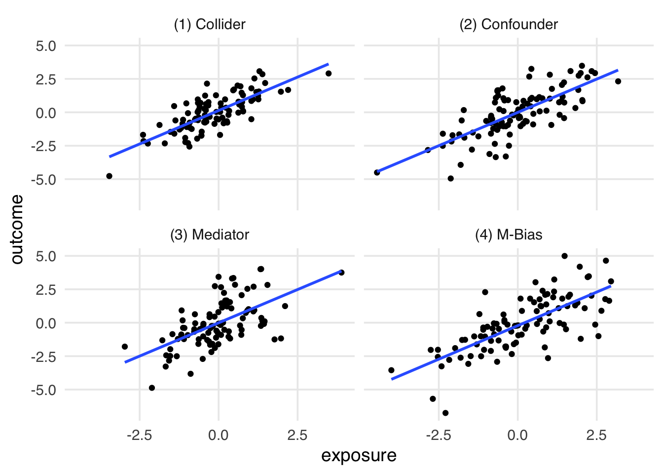
covariate. In the second dataset, covariate is a confounder, and we should control for it. In the third dataset, covariate is a mediator, and we should control for it if we want the direct effect, but not if we want the total effect.What can we do if the data can’t distinguish these causal structures? The best answer is to have a good sense of the data-generating mechanism. In Figure 6.7, we show the DAG for each dataset. Once we compile a DAG for each dataset, we only need to query the DAG for the correct adjustment set, assuming the DAG is right.
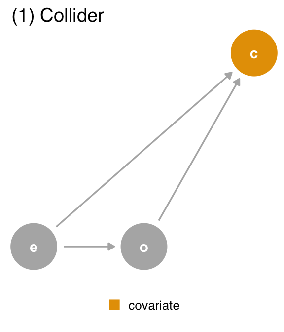
covariate (c) is a collider. We should not adjust for covariate, which is a descendant of exposure (e) and outcome (o).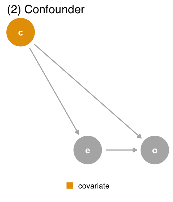
covariate (c) is a confounder. covariate is a mutual cause of exposure (e) and outcome (o), representing a backdoor path, so we must adjust for it to get the right answer.
covariate (c) is a mediator. covariate is a descendant of exposure (e) and a cause of outcome (o). The path through covariate is the indirect path, and the path through exposure is the direct path. We should adjust for covariate if we want the direct effect, but not if we want the total effect.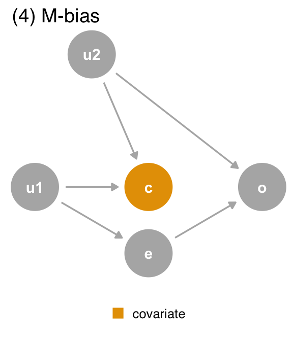
covariate (c) is a collider via M-Bias. Although covariate happens before both outcome (o) and exposure (e), it’s still a collider. We should not adjust for covariate, particularly since we can’t control for the bias via u1 and u2, which are unmeasured.The data generating mechanism1 in the DAGs matches what generated the datasets, so we can use the DAGs to determine the correct effect: unadjusted in datasets 1 and 4 and adjusted in dataset 2. For dataset 3, it depends on which mediation effect we want: adjusted for the direct effect and unadjusted for the total effect.
| Data generating mechanism | Correct causal model | Correct causal effect |
|---|---|---|
| (1) Collider | outcome ~ exposure | 1 |
| (2) Confounder | outcome ~ exposure; covariate | 0.5 |
| (3) Mediator | Direct effect: outcome ~ exposure; covariate, Total Effect: outcome ~ exposure | Direct effect: 0, Total effect: 1 |
| (4) M-Bias | outcome ~ exposure | 1 |
Hopefully, we have convinced you of the usefulness of DAGs. However, constructing correct DAGs is a challenging endeavor. In the causal quartet, we knew the DAGs because we generated the data. We need background knowledge to assemble a candidate causal structure in real life. For some questions, such background knowledge is not available. For others, we may worry about the complexity of the causal structure, particularly when variables mutually evolve with each other, as in Figure 5.26.
One heuristic is particularly useful when a DAG is incomplete or uncertain: time. Because causality is temporal, a cause must precede an effect. Many, but not all, problems in deciding if we should adjust for a confounder are solved by simply putting the variables in order by time. Time order is also one of the most critical assumptions you can visualize in a DAG, so it’s an excellent place to start, regardless of the completeness of the DAG.
Consider Figure 6.8 (a), a time-ordered version of the collider DAG where the covariate is measured at both baseline and follow-up. The original DAG actually represents the second measurement, where the covariate is a descendant of both the outcome and exposure. If, however, we control for the same covariate as measured at the start of the study (Figure 6.8 (b)), it cannot be a descendant of the outcome at follow-up because it has yet to happen. Thus, when you are missing background knowledge as to the causal structure of the covariate, you can use time-ordering as a defensive measure to avoid bias. Only control for variables that precede the outcome.
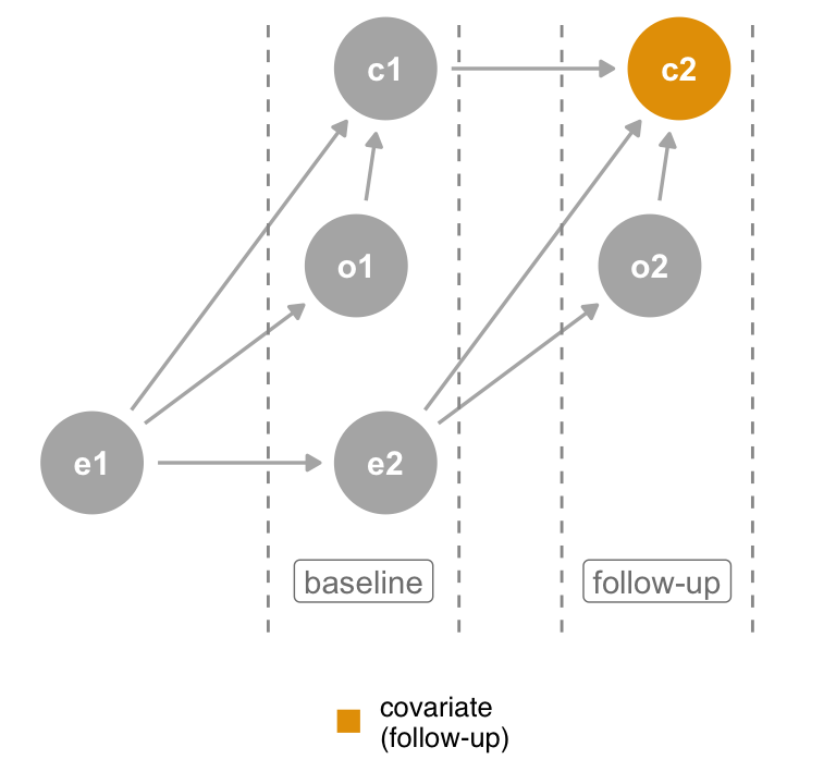
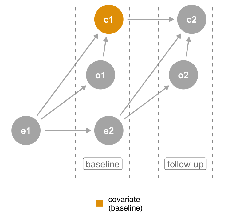
covariate at follow-up is a collider, but controlling for covariate at baseline is not.The time-ordering heuristic relies on a simple rule: don’t adjust for the future.
The quartet package’s causal_quartet_time has time-ordered measurements of each variable for the four datasets. Each has a *_baseline and *_follow-up measurement.
causal_quartet_time# A tibble: 400 × 12
covariate_baseline exposure_baseline
<dbl> <dbl>
1 -0.0963 -1.43
2 -1.11 0.0593
3 0.647 0.370
4 0.755 0.00471
5 1.19 0.340
6 -0.588 -3.61
7 -1.13 1.44
8 0.689 1.02
9 -1.49 -2.43
10 -2.78 -1.26
# ℹ 390 more rows
# ℹ 10 more variables: outcome_baseline <dbl>,
# covariate_followup <dbl>, exposure_followup <dbl>,
# outcome_followup <dbl>, exposure_mid <dbl>,
# covariate_mid <dbl>, outcome_mid <dbl>, u1 <dbl>,
# u2 <dbl>, dataset <chr>Using the formula outcome_followup ~ exposure_baseline + covariate_baseline works for three out of four datasets. Even though covariate_baseline is only in the adjustment set for the second dataset, it’s not a collider in two of the other datasets, so it’s not a problem.
| Dataset | Adjusted effect | Truth |
|---|---|---|
| (1) Collider | 1.00 | 1.00 |
| (2) Confounder | 0.50 | 0.50 |
| (3) Mediator | 1.00 | 1.00 |
| (4) M-Bias | 0.88 | 1.00 |
Where it fails is in dataset 4, the M-bias example. In this case, covariate_baseline is still a collider because the collision occurs before both the exposure and outcome. As we discussed in Section 5.3.2.1, however, if you are in doubt whether something is genuinely M-bias, it is better to adjust for it than not. Confounding bias tends to be worse, and meaningful M-bias is probably rare in real life. As the actual causal structure deviates from perfect M-bias, the severity of the bias tends to decrease. So, if it is clearly M-bias, don’t adjust for the variable. If it’s not clear, adjust for it.
Remember as well that it is possible to block bias induced by adjusting for a collider in certain circumstances because collider bias is just another open path. If we had u1 and u2, we could control for covariate while blocking potential collider bias. In other words, sometimes, when we open a path, we can close it again.
Predictive measurements also fail to distinguish between the four datasets. In Table 6.5, we show the difference in a couple of standard predictive metrics when we add covariate to the model. In each dataset, covariate adds information to the model because it contains associational information about the outcome 2. The RMSE goes down, indicating a better fit, and the R2 goes up, showing more variance explained. The coefficients for covariate represent the information about outcome it contains; they don’t tell us from where in the causal structure that information originates. Correlation isn’t causation, and neither is prediction. In the case of the collider data set, it’s not even a helpful prediction tool because you wouldn’t have covariate at the time of prediction, given that it happens after the exposure and outcome.
| Dataset | RMSE | R2 |
|---|---|---|
| (1) Collider | −0.14 | 0.12 |
| (2) Confounder | −0.20 | 0.14 |
| (3) Mediator | −0.48 | 0.37 |
| (4) M-Bias | −0.01 | 0.01 |
Relatedly, model coefficients for variables other than those of the causes we’re interested in can be difficult to interpret. In a model with outcome ~ exposure + covariate, it’s tempting to present the coefficient of covariate as well as exposure. The problem, as discussed Section 1.2.4, is that the causal structure for the effect of covariate on outcome may differ from that of exposure on outcome. Let’s consider a variation of the quartet DAGs with other variables.
First, let’s start with the confounder DAG. In Figure 6.9, we see that covariate is a confounder. If this DAG represents the complete causal structure for outcome, the model outcome ~ exposure + covariate will give an unbiased estimate of the effect on outcome for exposure, assuming we’ve met other assumptions of the modeling process. The adjustment set for covariate’s effect on outcome is empty, and exposure is not a collider, so controlling for it does not induce bias4. But look again. exposure is a mediator for covariate’s effect on outcome; some of the total effect is mediated through outcome, while there is also a direct effect of covariate on outcome. Both estimates are unbiased, but they are different types of estimates. The effect of exposure on outcome is the total effect of that relationship, while the effect of covariate on outcome is the direct effect.
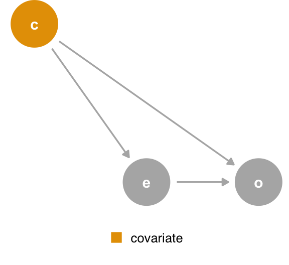
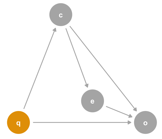
covariate is a confounder. If you look closely, you’ll realize that, from the perspective of the effect of covariate on the outcome, exposure is a mediator.What if we add q, a mutual cause of covariate and outcome? In Figure 6.10, the adjustment sets are still different. The adjustment set for outcome ~ exposure is still the same: {covariate}. The outcome ~ covariate adjustment set is {q}. In other words, q is a confounder for covariate’s effect on outcome. The model outcome ~ exposure + covariate will produce the correct effect for exposure but not for the direct effect of covariate. Now, we have a situation where covariate not only answers a different type of question than exposure but is also biased by the absence of q.
covariate is a confounder. Now, the relationship between covariate and outcome is confounded by q, a variable not necessary to calculate the unbiased effect of exposure on outcome.Specifying a single causal model is deeply challenging. Having a single model answer multiple causal questions is exponentially more difficult. If attempting to do so, apply the same scrutiny to both5 questions. Is it possible to have a single adjustment set that answers both questions? If not, specify two models or forego one of the questions. If so, you need to ensure that the estimates answer the correct question. We’ll also discuss joint causal effects in Chapter 16.
Unfortunately, algorithms for detecting adjustment sets for multiple exposures and effect types are not well-developed, so you may need to rely on your knowledge of the causal structure in determining the intersection of the adjustment sets.
See D’Agostino McGowan, Gerke, and Barrett (2023) for the models that generated the datasets.↩︎
For M-bias, including covariate in the model is helpful to the extent that it has information about u2, one of the causes of the outcome. In this case, the data generating mechanism was such that covariate contains more information from u1 than u2, so it doesn’t add as much predictive value. Random noise represents most of what u2 doesn’t account for.↩︎
If you recall, the Table Two Fallacy is named after the tendency in health research journals to have a complete set of model coefficients in the second table of an article. See Westreich and Greenland (2013) for a detailed discussion of the Table Two Fallacy.↩︎
Additionally, OLS produces a collapsable effect. Other effects, like the odds and hazards ratios, are non-collapsable, meaning you may need to include non-confounding variables in the model that cause the outcome in order to estimate the effect of interest accurately.↩︎
Practitioners of casual inference will interpret many effects from a single model in this way, but we consider this an act of bravado.↩︎